11 Shared concepts across three sites

An eigenvector is a direction learned from variation. An ontology concept is a named idea that people agree to reuse. “Databases” can remain a useful concept while a database-related news direction changes between archives. Linking the two would let a reader follow one subject through Eigen Times, Eigen Hacks, and Anthropology without pretending that the sites share one coordinate system.

This chapter separates three stages: the personal tags already implemented in the 2 October 2026 paper edition; a proposed, reviewed table connecting concepts to axes; and a proposed learned model whose predictions would require evaluation.

11.1 A tag, an axis, and a hierarchy

The ontology picker lets a reader choose a concept and attach its identifier to a canonical node. Searching a label and clicking it records an annotation. It does not rotate the news basis, retrain a person vector, or establish a public factual relationship.

The pinned ontology has 157 concepts in 11 areas; 61 concepts have multiple parents. This is a polyhierarchy: one concept can belong under several broader ideas. For an invented illustration, “distributed databases” might belong under both “databases” and “distributed systems.” These parent links describe meaning. They need not form perpendicular directions, and a person can have several tags at once.

An axis label serves a different purpose. Its strongest stemmed terms help a reader interpret one fitted direction. A list containing databas, ceo, and github does not define a clean databases category. Moreover, the negative pole needs inspection too: it is not automatically “not databases.” The sign of an eigenvector is a convention; a reviewed meaning must be attached to the appropriate pole and model version.

For the mechanics behind named directions, return to From eigenvectors to named axes.

11.2 A small, reviewed bridge comes first

A crosswalk is a table of correspondences. Imagine a proposed row saying: in this particular Eigen Hacks basis, the positive pole of this axis has useful evidence for the databases concept. The row should retain the corpus, axis and sign, basis fingerprint, ontology version, representative articles, method, and review status.

The bridge should be many-to-many. Several axes may help retrieve database articles, and one mixed axis may connect to several concepts. A reviewer can leave a proposed correspondence unassigned. Shared concept identifiers then become destinations across the three sites, while each route retains its original numerical coordinates.

Concept-to-concept mappings also have different strengths: “exact,” “close,” “broader,” “narrower,” and “related” do different jobs in the W3C SKOS mapping vocabulary. An axis would first need a reviewed semantic interpretation before those conceptual distinctions could be used responsibly. A familiar-looking word is insufficient.

11.3 Learning a concept score, one multiplication at a time

A later model could learn from reviewed articles. Let $m$ count the concepts reviewers label, and let $z$ be one article’s $1\times K$ standardized news row. Let $A$ be a $K\times m$ slope matrix: each slope measures how changing an input coordinate changes one concept’s linear score. Let $\beta$ be an $m\times1$ intercept column supplying baseline scores at zero input. The notation $\top$ is another form of the transpose symbol $\mathsf T$. Denote the resulting $1\times m$ prediction row by $s$. A simple linear predictor multiplies inputs by slopes and adds the baseline:

$$s=zA+\beta^\top.$$

Each column of $A$ asks how the news coordinates contribute to one concept. Its predictions are scores; no probability interpretation has yet been established.

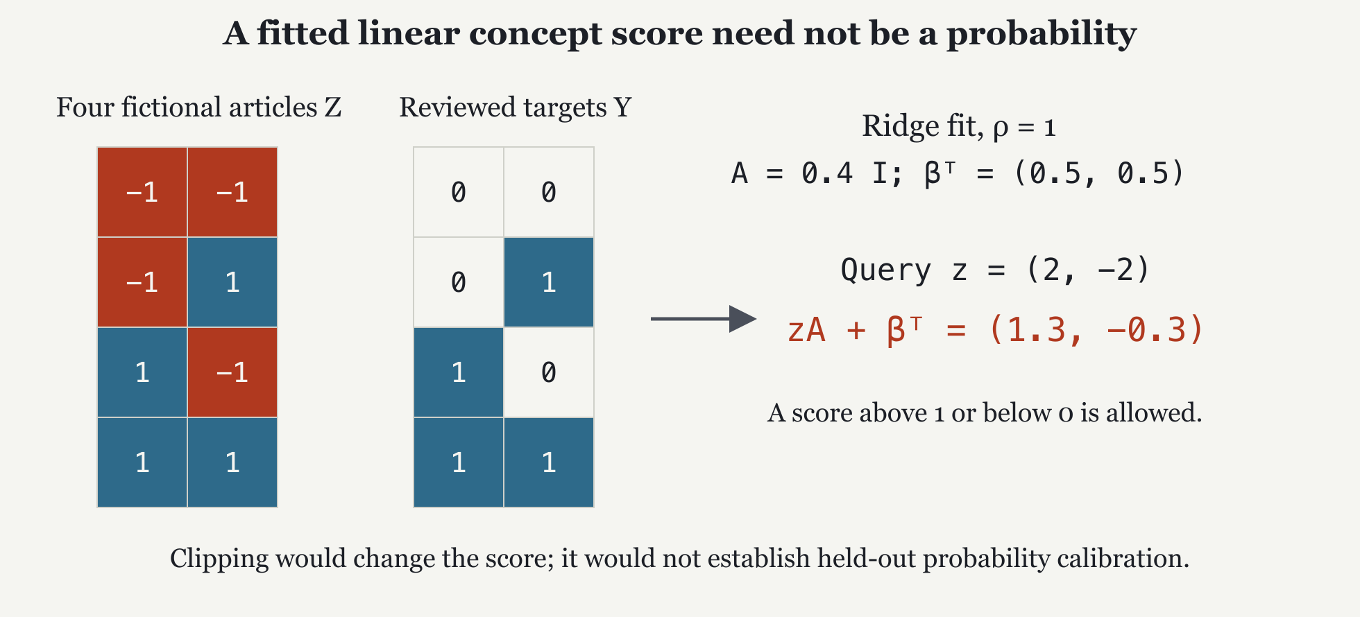
Consider an entirely illustrative two-coordinate, two-concept model:

$$\begin{aligned} z&=(2,-2),\\ A&=\begin{pmatrix}0.4&0\\0&0.4\end{pmatrix},\\ \beta^\top&=(0.5,0.5). \end{aligned}$$

The first prediction is $2(0.4)+(-2)(0)+0.5=1.3$. The second is $2(0)+(-2)(0.4)+0.5=-0.3$. Nothing went wrong when these escaped the interval zero to one: they are scores from an unconstrained linear rule. We have not made a probability model.

To learn the coefficients, let $N$ count reviewed training articles, distinct from the fitted-person count $n$ used earlier. Stack their standardized rows into the $N\times K$ matrix $Z$ and their matching concept labels into the $N\times m$ matrix $Y$. Row order agrees across the two matrices. For a binary label, an entry is one when reviewers judged the concept present and zero when they judged it absent. Missing judgments must remain missing, rather than becoming zeros.

A ridge fit balances squared prediction error against a penalty on large slopes. Let $\rho\ge0$ be the penalty strength. For a matrix, the Frobenius norm, denoted by double bars with subscript $F$, is the square root of the sum of squared entries. Thus its square adds those squared entries. Here $\mathbf1$ is a column of $N$ ones, so $\mathbf1\beta^\top$ repeats the baseline row for every article. The following objective assumes every target entry is observed; partially reviewed targets require a separately specified objective summing only observed errors. Choose $A$ and $\beta$ to minimize

$$\lVert ZA+\mathbf1\beta^\top-Y\rVert_F^2 +\rho\lVert A\rVert_F^2.$$

The first term adds squared prediction errors; the second penalizes large slopes. The intercept is deliberately unpenalized. A held-out validation procedure, using articles reserved from parameter fitting, would choose $\rho$ rather than a convenient-looking result on the training articles.

The toy coefficients above can actually be fitted. Take four fictional, fully reviewed article rows:

$$Z=\begin{pmatrix}-1&-1\\-1&1\\1&-1\\1&1\end{pmatrix},\qquad Y=\begin{pmatrix}0&0\\0&1\\1&0\\1&1\end{pmatrix}.$$

Each concept’s average label is 0.5, giving the intercept. Each coordinate column has sum of squares four and centered label-product sum two. With $\rho=1$, its fitted slope is $2/(4+1)=0.4$; the cross-slopes are zero. Training predictions are 0.1 or 0.9. The new row $(2,-2)$ then extrapolates beyond the training coordinates, producing $(1.3,-0.3)$. Training fit and behavior on new inputs are different tests.

Each corpus would need its own fitted coefficients. Shared target identifiers make the outputs comparable in meaning; they do not make the input bases interchangeable. Concepts overlap, so $A$ need not be orthogonal or even square. This semantic transformation does not inherit the reconstruction guarantees of $W$.

11.3.1 Derive the ridge slope instead of memorizing it

A derivative describes how a scalar output changes per small change in a scalar input. Start with a function $f(a)=a^2$, where $a$ is a real scalar, and let $\varepsilon$ be a nonzero change in that input. The difference quotient is

$$\frac{f(a+\varepsilon)-f(a)}{\varepsilon} =\frac{a^2+2a\varepsilon+\varepsilon^2-a^2}{\varepsilon} =2a+\varepsilon.$$

As $\varepsilon$ approaches zero, this approaches $2a$. That limiting slope is the derivative, written $f'(a)$. At $a=2$, changes of 0.1 and 0.01 give difference quotients 4.1 and 4.01, approaching 4. A derivative is a local rate of change; it is not the function’s output, which also happens to equal 4 at this particular input.

Return to the first ridge target. Its centered labels are $(-0.5,-0.5,0.5,0.5)$, and the first input coordinate is $(-1,-1,1,1)$. Temporarily call its scalar slope $a$ and set the other slope to zero. Each of the four squared prediction errors is $(a-0.5)^2$. With penalty $\rho=1$, the scalar objective, named $J(a)$, is

$$J(a)=4(a-0.5)^2+a^2=5a^2-4a+1.$$

Differentiate its expanded terms: $J'(a)=10a-4$. At an interior minimum a small move in either direction cannot improve the value, so the local slope must be zero. Solving $10a-4=0$ gives $a=0.4$. Complete the square to verify this is a minimum: $J(a)=5(a-0.4)^2+0.2$. Its minimum value is 0.2. At $a=0$ the value is 1; at $a=0.5$ it is 0.25. Ridge accepts a little prediction error to reduce the coefficient penalty.

For any nonnegative penalty $\rho$, this example instead has derivative $2(4+\rho)a-4$, giving $a=2/(4+\rho)$. The input columns have zero cross-product, so the two slopes separate cleanly. In a general table they interact. Let $Z_c$ subtract each input column mean from $Z$, and let $Y_c$ subtract each target column mean from $Y$. Let $I$ here be the $K\times K$ identity. The stationary equations for these centered tables are $(Z_c^{\mathsf T}Z_c+\rho I)A=Z_c^{\mathsf T}Y_c$. Solving this equation finds the slopes; restoring the target means minus the mean input’s fitted contribution gives the unpenalized intercepts.

The notation $\partial J/\partial a$ denotes a partial derivative: change coefficient $a$ while holding the other coefficients fixed. The gradient collects all those partial derivatives in the coefficient table’s shape. For the full squared-error objective its slope gradient is $2[Z_c^{\mathsf T}(Z_cA-Y_c)+\rho A]$. Setting the whole gradient to zero yields the same stationary equations. The notebooks check the scalar derivative with small finite changes, the completed-square minimum, and the fitted matrix equations independently.

11.4 A score becomes a probability only after another question

First define what is being predicted. One possible event is: “Under this annotation protocol, reviewers judge that this article substantially discusses databases.” It is not “this person is a database person.”

A logistic predictor maps a linear score through a smooth S-shaped function whose output lies between zero and one. Calibration means agreement between predicted probabilities and observed frequencies; the logistic bound alone does not establish it. The distinction is developed in Guo and colleagues’ study of calibration.

A reliability diagram offers a simple check. In an invented test set, collect 100 articles assigned probabilities near 0.8. Suppose reviewers mark 55 as positive. Plot their mean prediction near 0.8 horizontally and the observed fraction 0.55 vertically. A well-calibrated bin would lie near the diagonal, where those numbers agree. This example is hypothetical; Anthropology has not reported such a calibration experiment.

Repeat across probability ranges, report the number of articles in each bin and uncertainty, and inspect relevant sources and periods separately. Small bins can fluctuate substantially. Prevalence is the fraction of articles with a positive target. A model that predicts this overall fraction for every article can be calibrated yet poor at ranking individual articles. Discrimination is its ability to distinguish positive from negative cases. Calibration and discrimination therefore need separate evaluation, with articles reserved for testing rather than reused for fitting or tuning.

Checkpoint. The toy linear model predicts 1.3. Can the interface print “130% confidence”? Answer: No. It can display a labeled score. A probability needs a defined target, a suitable model, and held-out evidence that its estimates behave like probabilities.

11.4.1 Work through the logistic function and one fitting step

Let $t$ denote a real-valued linear score and let $p$ denote a modeled probability for one defined binary article label. Write $\exp(t)=e^t$ for the exponential function, with base $e\approx2.71828$; its output is positive for every finite real input. The logistic function, written $\sigma(t)$ in this section only, is

$$p=\sigma(t)=\frac{1}{1+\exp(-t)}.$$

At zero, $\exp(0)=1$, so $\sigma(0)=1/2$. At two, $\exp(-2)\approx0.135335$, so $\sigma(2)\approx0.880797$. At minus two, $\sigma(-2)\approx0.119203$. The denominator always exceeds one, placing the result strictly between zero and one for finite scores. This function’s $\sigma$ is not the earlier standard deviation $\sigma_j$.

To fit such outputs, the notebook uses the first column of the four-row target table. Let $\theta$ be a two-entry slope column and $b_0$ a scalar intercept, giving score $t_i=z_i\theta+b_0$ for training article index $i$. Let $y_i$ be its reviewed zero-or-one target. Binary log loss for one row is $-y_i\log p_i-(1-y_i)\log(1-p_i)$, where $\log$ is the natural logarithm, the inverse of the exponential. A correct high-probability prediction gets a small loss; a confidently wrong one gets a large loss. All four losses are averaged. The demonstration adds $\eta\lVert\theta\rVert^2/2$ with penalty $\eta=0.1$, keeping the intercept unpenalized.

We need three derivative rules before differentiating this model. The derivative of $\exp(t)$ is $\exp(t)$; the derivative of $\log p$ is $1/p$ for positive $p$; and the derivative of the reciprocal $1/q$ with respect to nonzero $q$ is $-1/q^2$. The chain rule multiplies the local rates when one function is placed inside another. We use these rules here and verify the resulting derivatives by small finite changes in the notebooks.

To differentiate the logistic function, name its denominator $q(t)=1+\exp(-t)$. The inner negative sign has derivative -1, so $q'(t)=-\exp(-t)$. Applying the reciprocal rule and the chain rule gives

$$\sigma'(t)=-\frac{q'(t)}{q(t)^2} =\frac{\exp(-t)}{(1+\exp(-t))^2}.$$

One factor is $p=1/(1+\exp(-t))$; the other is $1-p=\exp(-t)/(1+\exp(-t))$. Hence the derivative is $p(1-p)$. At $t=0$, its value is $(1/2)(1/2)=1/4$.

Now let $\mathcal L(p)$ name a single row’s log loss and let $y$ be its fixed binary target. The notation $d\mathcal L/dp$ writes its derivative with respect to $p$. Differentiating with respect to its probability gives

$$\begin{aligned} \frac{d\mathcal L}{dp}&=-\frac{y}{p}+\frac{1-y}{1-p}\\ &=\frac{-y(1-p)+(1-y)p}{p(1-p)}\\ &=\frac{p-y}{p(1-p)}. \end{aligned}$$

Composing this loss with the logistic score multiplies by $dp/dt=p(1-p)$, cancelling the denominator and leaving $d\mathcal L/dt=p-y$. A slope changes the score at a rate equal to its input coordinate; the intercept changes it at rate one. Thus the slope gradient is the average of $z_i^{\mathsf T}(p_i-y_i)$ plus $\eta\theta$; the intercept gradient is the average of $p_i-y_i$.

Start all slopes and the intercept at zero. Every prediction is 0.5, so the four errors are $(0.5,0.5,-0.5,-0.5)$. Multiplying those by the first input column and averaging gives $(-0.5-0.5-0.5-0.5)/4=-0.5$. The second slope gradient and intercept gradient are both zero. A gradient-descent step subtracts the gradient times a positive step size; with step size 0.2 the new slopes are $(0.1,0)$ and the intercept stays zero. Positive first-coordinate articles now receive $\sigma(0.1)\approx0.524979$.

The native notebooks repeat that update 2,000 times and check a small final gradient and a separate reference slope. This verifies the training calculation for declared synthetic inputs. It supplies no real-world held-out calibration result. In the separate hypothetical reliability bin, $55/100=0.55$ observed frequency differs from 0.8 predicted frequency by 0.25. Constraining outputs to a probability range and testing their agreement with observations remain distinct tasks.

11.5 Why an article model cannot simply label a person

A person profile $b$ has been background-adjusted and normalized. It describes the direction of distinctive coverage. An article row $z$ has undergone neither of those person-level operations. Their equal number of coordinates does not make them the same kind of observation.

For a person score row $u$, the earlier chapters reconstructed an approximate profile as $\overline b+uW^\top$. Use the people basis and article predictor from the same corpus and news-coordinate version. Let $s_{\mathrm{person}}$ denote the $1\times m$ score row obtained by applying the article predictor to this reconstructed profile. Substitution gives

$$s_{\mathrm{person}}=\overline b A+\beta^\top+u(W^\top A).$$

The product $W^\top A$ has shape $r\times m$: it describes how moving along each of the $r$ people directions would change those linear scores. This is a valid algebraic identity. Its interpretation as a useful prediction about a person remains an untested use outside the article model’s training distribution. Neither restoring the mean nor adding the intercept solves that problem.

Another possible quantity is the fraction of a person’s associated articles predicted to discuss a concept. That answers a coverage question, with uncertainty from both article attribution and classification. For a nonlinear predictor, predicting an average row and averaging individual predictions can differ. A future system must specify which quantity it means and evaluate it on independently reviewed person-level examples.

11.5.1 Check the algebra and then the meaning

Substitute the reconstructed row into the article rule directly: $(\bar b+uW^{\mathsf T})A+\beta^{\mathsf T}$. Distribute multiplication over addition to obtain $\bar bA+uW^{\mathsf T}A+\beta^{\mathsf T}$, then group the last matrix product as $u(W^{\mathsf T}A)$. Grouping changes where we calculate intermediate tables, without changing their compatible dimensions or result. The notebook uses a separately declared three-input, two-output synthetic slope table because the earlier two-input ridge table does not fit the three-coordinate people fixture.

For a nonlinear example, take scalar article scores zero and two. Their average is one, so predicting after averaging gives $\sigma(1)\approx0.731059$. Predicting separately and then averaging gives $(\sigma(0)+\sigma(2))/2=(0.5+0.880797)/2\approx0.690399$. The difference is approximately 0.040660. Thus even the arithmetic choice of when to aggregate changes the output. A defined person-level target and separately reviewed evaluation remain necessary whichever quantity is chosen.

11.6 Aligning maps needs anchors and room to test them

Suppose two corpora contain reviewed representations of the same people. An anchor is a pair of rows known to describe the same entity in the two corpora. An orthogonal Procrustes fit tries to rotate or reflect one set of such rows toward the other. For this alignment only, let $M$ count paired anchors and $k$ count coordinates in each representation. Let $X$ and $Y$ be their centered $M\times k$ tables, with matching entities in the same row; $Y$ here is an anchor table, not the preceding concept-target matrix. Let $Q_{\mathrm{align}}$ be a $k\times k$ alignment matrix, distinct from the SVD factor $Q$. The identity $I$ now has shape $k\times k$. The fit minimizes $\lVert XQ_{\mathrm{align}}-Y\rVert_F^2$ subject to the orthogonality constraint $Q_{\mathrm{align}}^\top Q_{\mathrm{align}}=I$.

The constraint preserves distances within the chosen coordinate geometry. It cannot correct every difference in populations, source coverage, or scaling. Shared names are not enough; the anchors must be correctly identified and substantively comparable.

The published models share 60 canonical people. Sixty centered rows in 60 dimensions have rank at most 59: subtracting their mean makes the rows sum to zero, creating a dependence. Consequently, they cannot determine a full 60-dimensional alignment from independent evidence in every direction. Reserving anchors for testing leaves still fewer for fitting. A lower-dimensional or regularized approach is possible, but its assumptions and performance need evaluation. See Matching axes for the prerequisite distinction between comparing directions and assigning correspondences.

11.6.1 Fit an exact toy alignment and reserve a test row

Use four centered synthetic anchor rows $(-1,-1)$, $(-1,1)$, $(1,-1)$, and $(1,1)$ for $X$. Stipulate a known map $\begin{pmatrix}0&-1\\1&0\end{pmatrix}$ only to construct test data $Y$. It maps a row $(a,b)$ to $(b,-a)$. The first pair is therefore $(-1,-1)$ and $(-1,1)$. The two tables have zero column means.

For the fit, multiply paired columns to obtain $X^{\mathsf T}Y=\begin{pmatrix}0&-4\\4&0\end{pmatrix}$. Denote the SVD of this product by $L\Sigma_{\mathrm{align}}T^{\mathsf T}$, where $L$ and $T$ are two-by-two orthogonal direction matrices and $\Sigma_{\mathrm{align}}$ contains its nonnegative singular values. The Procrustes solution is $Q_{\mathrm{align}}=LT^{\mathsf T}$. The notebook computes it from the paired tables, then checks that it equals the stipulated map and gives zero training discrepancy.

Why this choice? Expanding the squared discrepancy yields the squared lengths of $X$ and $Y$ minus twice the trace of $Q_{\mathrm{align}}^{\mathsf T}X^{\mathsf T}Y$. The first two quantities are fixed under an orthogonal map. In the singular coordinate frame, the trace is largest when each nonnegative singular value is multiplied by one rather than a smaller diagonal coefficient of an orthogonal matrix. The choice $LT^{\mathsf T}$ achieves that maximum, and therefore the minimum discrepancy. This permits reflections as well as rotations, exactly as the stated constraint allows.

Reserve a fifth row $(0.3,-0.7)$ from fitting. Its stipulated target is $(-0.7,-0.3)$; the estimated map reproduces that target with zero error. This noiseless test proves the toy algebra, not a real alignment’s usefulness. Actual held-out anchors could disagree because coverage, scale, or meaning differs between corpora.

The rank shortage has an equally small example. Center three two-coordinate rows: their sum becomes $(0,0)$, so the third row is the negative sum of the first two. There are at most two independent centered rows. With sixty centered anchors, the same dependence leaves at most fifty-nine independent rows. The notebooks also compute this bound using a synthetic centered sixty-by-sixty identity table; it is not a measurement of the real anchor matrix.