5 The singular value decomposition and LSA

5.1 What the SVD is

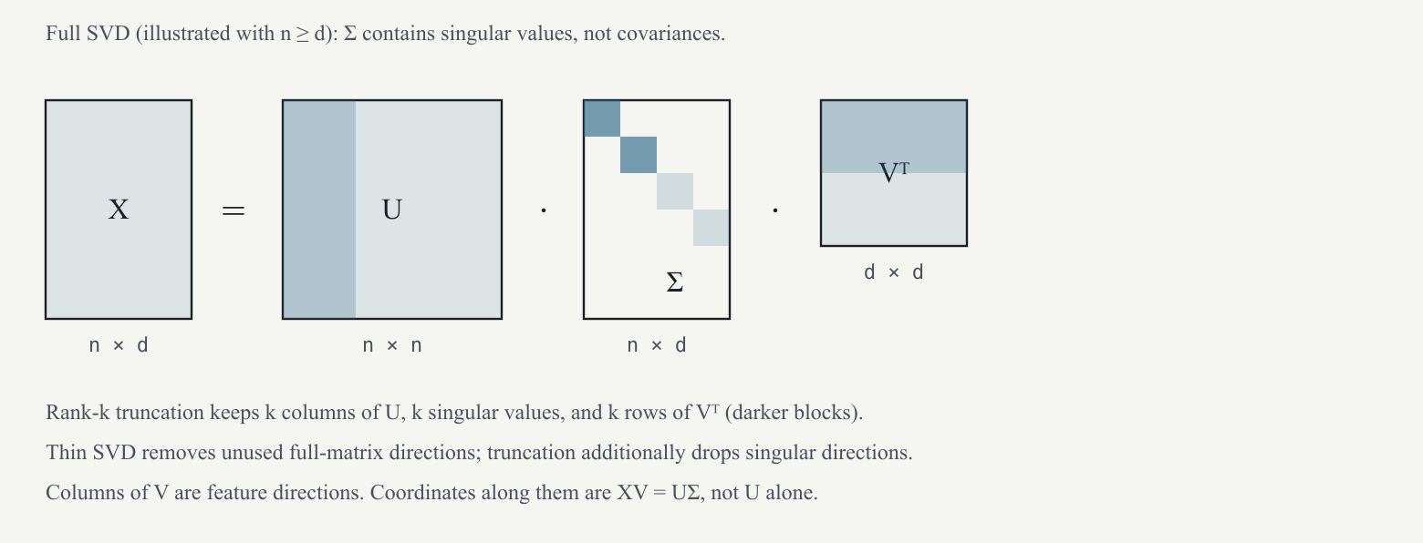
The eigendecomposition works on a square covariance. The singular value decomposition (SVD) works directly on a rectangular data matrix. It separates a matrix operation into input directions, nonnegative scale factors, and output directions. The input and output can have different dimensions, so the directions on the two sides need not live in the same space.

5.1.1 Follow one input direction through a rectangular table

For this chapter let $X$ be any $n\times d$ matrix. A column input has $d$ entries and the output $Xv$ has $n$ entries. In the small example

$$X=\begin{pmatrix}3&0\\0&2\\0&0\end{pmatrix},$$

the input $(1,0)^{\top}$ maps to $(3,0,0)^{\top}$, which is three times the unit output direction $(1,0,0)^{\top}$. The input $(0,1)^{\top}$ maps to $(0,2,0)^{\top}$, which is twice $(0,1,0)^{\top}$. These perpendicular input directions map to perpendicular output directions, with scale factors 3 and 2. The output has three entries even though the input has two.

For a general matrix, SVD finds suitable directions even when the input table is not already diagonal. Let $v_j$ be a unit right singular direction in the input space, let $u_j$ be its unit left singular direction in the output space, and let $\sigma_j$ be their nonnegative scale. The key relation is $Xv_j=\sigma_ju_j$. “Right” and “left” describe where the directions appear in the factorization; neither means an orientation on a page. A zero scale contributes no output in that direction.

5.1.2 Assemble the separate directions into matrices

Let $U$ be an $n\times n$ orthogonal matrix of left directions, and $V$ a $d\times d$ orthogonal matrix of right directions. Let $\Sigma_{\mathrm{svd}}$ be an $n\times d$ rectangular diagonal matrix: its only potentially nonzero entries lie where row and column indices agree. Those entries are the singular values $\sigma_j$ in decreasing order. Then

$$X=U\Sigma_{\mathrm{svd}}V^{\top}.$$

Figure 6 labels this singular-value matrix with the traditional bare $\Sigma$; it is a different object from the covariance $\Sigma$ in §4. The columns of $V$ are directions indexed by features, and those of $U$ are directions indexed by observations. Actual coordinate scores are $XV=U\Sigma_{\mathrm{svd}}$, not $U$ alone: each left direction must receive its singular-value scale.

Read the product from right to left, as with eigendecomposition. $V^{\top}$ resolves an input into right-direction coordinates; $\Sigma_{\mathrm{svd}}$ scales those coordinates and accounts for the change in dimension; $U$ writes the result in the original output coordinates. For the $3\times2$ example, full factors can use a $3\times3$ identity for $U$, a $2\times2$ identity for $V$, and the displayed rectangular table for $\Sigma_{\mathrm{svd}}$. Nothing needs turning because the table already uses suitable directions.

Let $q=\min(n,d)$, where $\min$ selects the smaller number. The thin SVD removes the unused full-matrix directions: it has $U$ of shape $n\times q$, $\Sigma_{\mathrm{svd}}$ of shape $q\times q$, and $V$ of shape $d\times q$, with the same product $X$. Keeping only $k<q$ directions is the further operation of truncation.

In the example, $q=2$. The thin $U$ keeps the first two columns of the three-dimensional identity, the scale matrix becomes $\mathrm{diag}(3,2)$, and $V$ remains the two-dimensional identity. Multiplying these factors still reconstructs every entry. Thin factorization changes storage without losing any information; truncation will deliberately lose contributions.

5.1.3 Why covariance eigenvalues contain squared singular values

Transposing a product reverses its order: $(AB)^{\top}=B^{\top}A^{\top}$. Apply that rule to the SVD, multiply, and use $U^{\top}U=I$. For the full rectangular decomposition the steps are

$$X^{\top}X =V\Sigma_{\mathrm{svd}}^{\top}U^{\top}U\Sigma_{\mathrm{svd}}V^{\top} =V(\Sigma_{\mathrm{svd}}^{\top}\Sigma_{\mathrm{svd}})V^{\top}.$$

Each diagonal entry in the middle is a singular value multiplied by itself. For the thin decomposition the middle product is the square diagonal matrix $\Sigma_{\mathrm{svd}}^2$. Thus the right singular directions are also eigenvectors of the Gram matrix, with squared singular values as eigenvalues. In the exact example, the Gram matrix is $\mathrm{diag}(9,4)$.

If $X$ is centered and equally weighted, covariance is that Gram matrix divided by $n$. Its right directions therefore stay the same, and its eigenvalues are $\lambda_j=\sigma_j^2/n$. The diagonal example above is not centered, so its Gram matrix should not silently be called an empirical centered covariance. The notebook also applies the identity to the centered six-document table.

For the weighted covariance of §4, instead decompose $W^{1/2}X_c$. Here $W^{1/2}$ is diagonal with entries $\sqrt{w_i}$, so it scales each centered row by the square root of its weight. When we form a Gram product, one square-root weight comes from each factor; their product is the full weight $w_i$. Divide the resulting squared singular values by total weight $Z$. Scores for the original, unweighted observations are still $X_cV$, not the weighted rows’ scores. A direction’s canon is its representative collection of high-scoring stories; a left singular vector alone is not generally the original article-score column in a weighted fit.

5.2 Truncation

Let $U_k$ and $V_k$ contain the first $k$ columns of the thin factors, and let $\Sigma_k$ contain their $k$ singular values on its diagonal. Their shapes are $n\times k$, $d\times k$, and $k\times k$, respectively. The approximation $X_k=U_k\Sigma_kV_k^{\top}$ has rank at most $k$. It keeps only $k$ independent contributions with which to rebuild the table.

5.2.1 Measure what a reconstruction leaves behind

The residual table is original minus reconstructed, $X-X_k$. A positive residual entry says that the reconstruction was smaller than the original there; a negative entry says it was larger. Adding those signed errors would allow overestimates and underestimates to cancel. Instead square every entry and add. This is the sum of squared errors. Least squares means choosing a reconstruction that makes such a sum as small as the allowed family permits.

The Frobenius norm, written $\lVert A\rVert_F$ for a matrix $A$, is the square root of the sum of all its squared entries. It extends vector length to a whole table by treating every cell as a coordinate. Minimizing this norm or its square gives the same minimizing table, because the square-root function preserves order among nonnegative numbers.

In the rectangular diagonal example, keeping the scale 3 and dropping the scale 2 reconstructs only the entry 3. The residual has a single nonzero entry, 2. Its squared Frobenius norm is therefore 4, and its norm is 2. The original table’s squared norm is $9+4=13$. Define relative error as residual norm divided by the positive original norm; here it is $2/\sqrt{13}\approx0.5547$. An error ratio is not a proportion of articles reconstructed correctly; it compares geometric lengths in this representation.

5.2.2 A small detour: what minimizing and differentiating mean

Before asking a matrix theorem to minimize anything, solve a scalar fitting problem. Suppose we must replace the observations 1, 2, and 3 by one common fitted value, called $\theta$ (Greek theta). Their residuals are $1-\theta$, $2-\theta$, and $3-\theta$. Let $J(\theta)$ name their sum of squared residuals; $J$ is a function, a rule returning a number for each proposed input $\theta$. Expanding the three squares gives

$$\begin{aligned} J(\theta)&=(1-\theta)^2+(2-\theta)^2+(3-\theta)^2\\ &=3\theta^2-12\theta+14\\ &=3(\theta-2)^2+2. \end{aligned}$$

The last form makes the minimum visible. A square cannot be negative, and $(\theta-2)^2$ is zero exactly when $\theta=2$. Thus the smallest squared error is 2. Trying $\theta=1$ or $\theta=3$ gives squared error 5. At the best fit the signed residuals are −1, 0, and 1; their sum is zero, while their sum of squares is two. These are different quantities.

Differentiation provides another way to inspect how changing the fit changes the error. Let $h$ be a small nonzero change in $\theta$. The difference $J(\theta+h)-J(\theta)$ is the change in error. Divide by $h$ to obtain change in error per unit change in the fitted value, an average slope over that step. Expanding the quadratic and canceling equal terms gives

$$\frac{J(\theta+h)-J(\theta)}{h}=6\theta-12+3h.$$

As the step becomes arbitrarily small, the last term approaches zero. The resulting local slope is the derivative, written $J'(\theta)$ or $\mathrm{d}J/\mathrm{d}\theta$; the prime here means derivative, not the rotated coordinate notation used later:

$$J'(\theta)=6\theta-12.$$

We differentiated to learn which way the error changes. Below 2 the slope is negative, so increasing the fit locally lowers error; above 2 the slope is positive, so increasing it locally raises error. At 2 the slope is zero. A zero derivative is a stationary point, not automatically a minimum for every function. Here the completed-square formula proves it is the global minimum. This example supplies the meaning of derivative, the calculation from a small change, and the reason for setting it to zero. No matrix differentiation is required to use the SVD that follows.

5.2.3 The best reconstruction within a rank budget

The Eckart–Young theorem says that the truncated SVD minimizes $\lVert X-X_k\rVert_F$ among all matrices of rank at most $k$. This comparison matters: we are not saying that an arbitrary reconstruction is best, or that the reconstruction is a true explanation of the subjects. We are choosing the best approximation under this particular squared-error measure and rank constraint.

The squared error equals the sum of squared discarded singular values. To see the accounting, each singular component has a unit left direction, a unit right direction, and a scale $\sigma_j$. Its contribution to squared table length is $\sigma_j^2$. Distinct components are perpendicular when their tables are compared entry by entry, so their squared lengths add without cross terms. Keeping the largest scales retains the most of this length budget. The theorem adds the stronger claim that no different rank-$k$ table does better.

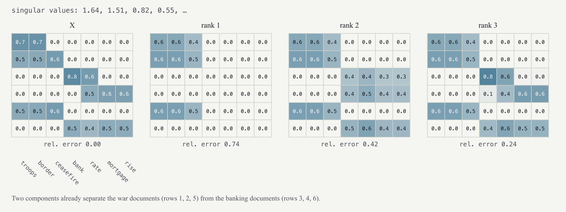
Figure 7 applies this to the six-document matrix of Figure 1. Its singular values are 1.64, 1.51, 0.82, 0.55, and then almost nothing. Relative error means $\lVert X-X_k\rVert_F/\lVert X\rVert_F$ for nonzero $X$. Compute it by squaring and adding the discarded singular values, dividing by the sum of all squared singular values, and taking a square root. Rank 1 rebuilds only the war documents (relative error 0.74); rank 2 rebuilds both blocks, war and banking, and the error drops to 0.42; rank 3 reaches 0.24. Two components already separate the two kinds of document in this small example. The notebook uses unrounded singular values, so its checks do not accumulate rounding error from the printed labels.

5.3 Latent semantic analysis

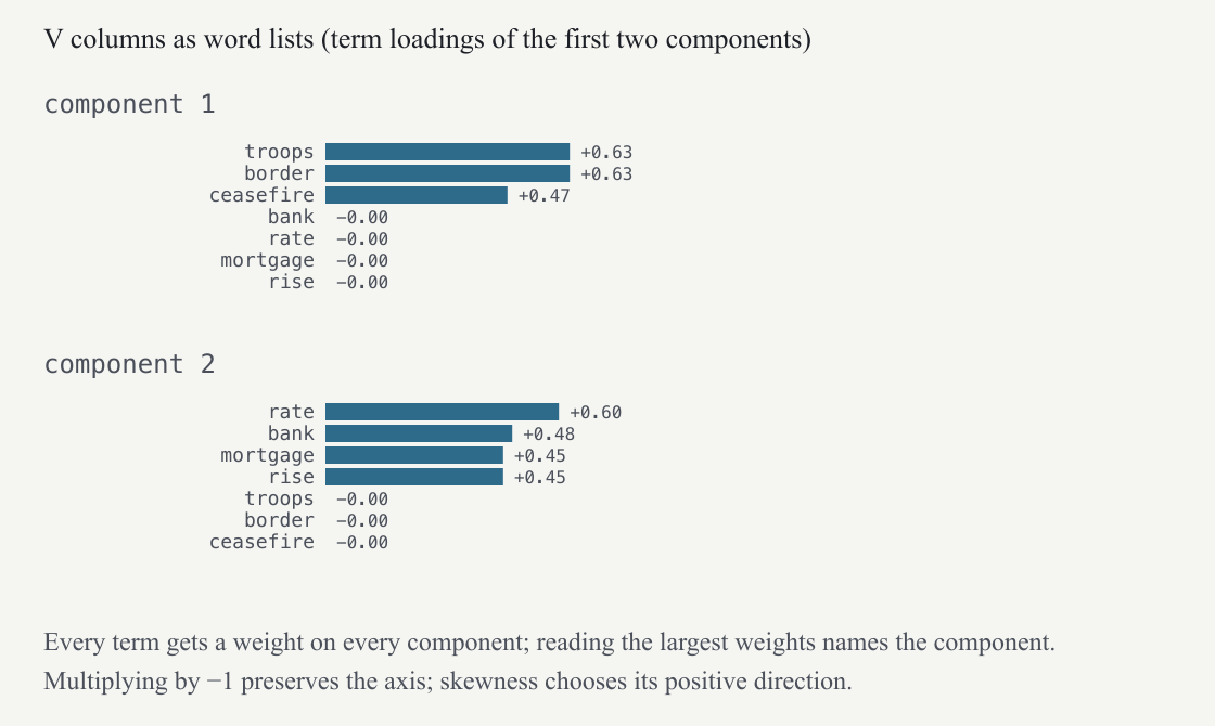
Latent semantic analysis (LSA) uses a truncated SVD of a document–term matrix such as TF‑IDF; Eigen Times additionally centres and, in the archive edition, weights that matrix. Each retained column of $V$ is a direction over terms. Its entries are loadings: coefficients telling how strongly each input feature contributes to the direction. Its largest term loadings provide a word list (Figure 8). In the toy corpus the first component loads on troops, border, ceasefire, the second on bank, rate, mortgage, rise. In the real Eigen Times v0 basis the axes read bank · financial · credit · rate · loan, Russian · Russia · Ukraine · Putin · Moscow, flight · airline · passenger · airport · crash, and so on—sixty word lists that a reader recognises at once.

There are two distinct roles for a loading. When measuring an article’s coordinate, multiply each term entry by the direction’s loading for that term, then add the products. When reconstructing an article, multiply that whole direction by the article’s coordinate on it. A loading’s sign determines which pole of the direction it supports; its magnitude measures strength within this numerical representation. Neither alone is a probability that a document concerns a subject. A word list is a reading aid extracted from the direction, not a replacement for its full vector.

The small factorization can be computed directly. The real document–term table needs two additional ideas: applying a centered table without storing it, and finding its leading directions through a much smaller working space. We develop them separately.

5.3.1 Apply centering without storing a dense centered table

For this calculation, $X$ has $n$ document rows and $p$ term columns, $\mu$ is its $p\times1$ reference mean, and $\mathbf1$ has $n$ entries. Forming $X_c=X-\mathbf1\mu^{\top}$ would turn many absent-term zeros into negative mean values and destroy sparsity. We can still calculate a product involving $X_c$ without storing those changed cells.

Let $l$ count a small number of working columns, let $\Omega$ (capital omega) be any $p\times l$ matrix, and let $Y$ be $n\times l$. Each column of $\Omega$ is an input direction. Expand the centered product using the rule that multiplication distributes over subtraction:

$$X_c\Omega=(X-\mathbf1\mu^{\top})\Omega =X\Omega-(\mathbf1\mu^{\top})\Omega.$$

Associativity lets us change the grouping in the last product without changing its order. Compute the small $1\times l$ row $\mu^{\top}\Omega$ first, then repeat that row $n$ times using $\mathbf1$. For the transposed operation, apply the same reasoning. The resulting identities are

$$X_c\Omega=X\Omega-\mathbf1(\mu^{\top}\Omega),$$ $$X_c^{\top}Y=X^{\top}Y-\mu(\mathbf1^{\top}Y).$$

The results have shapes $n\times l$ and $p\times l$. In the second correction, $\mathbf1^{\top}Y$ adds each column of $Y$ over observations; multiplying those column totals by $\mu$ constructs the needed adjustment. Each correction is an outer product, of rank at most one, because all its columns are scalar multiples of the same column. The sparse $X$ is used as is; the centered dense matrix need never be stored. The notebook verifies both identities against a directly centered small table before using them in the larger algorithm.

5.3.2 Build a small working space

A $1{,}093{,}166\times50{,}000$ matrix is far too large for a full classical SVD here, but only the top 60 directions are wanted. The method of Halko, Martinsson and Tropp approximates them with repeated matrix products. Draw a random $50{,}000\times80$ matrix $\Omega$: $l=80$ working columns provide $k=60$ desired directions plus 20 extra directions for approximation. Each random column mixes many input features; applying $X_c$ gives one corresponding mixture of output directions. The resulting $n\times l$ table $Y=X_c\Omega$ is called a sketch: a smaller collection of vectors with which to explore the large matrix’s output space. The extra columns are oversampling, a margin for approximation rather than extra final news axes.

The range of a matrix is the set of outputs it can produce. The goal is for the sketch’s span to cover the most important part of that range. Random combinations can capture the leading directions well when the singular values decay sufficiently; the method offers an approximation whose quality must still be assessed.

5.3.3 Make the working directions perpendicular

To orthonormalise is to replace spanning vectors by perpendicular unit vectors spanning the same space. Here is one step of the Gram–Schmidt idea used to explain that operation. Take columns $a=(1,1)^{\top}$ and $b=(1,0)^{\top}$. First normalize $a$ to the unit column $q_1=a/\sqrt2$. The scalar $q_1^{\top}b=1/\sqrt2$ measures how much of $b$ already lies along $q_1$. The corresponding vector contribution is $q_1(q_1^{\top}b)=(1/2,1/2)^{\top}$.

Subtract that contribution from $b$. The residual is $(1/2,-1/2)^{\top}$ and has dot product zero with $q_1$. Normalize it to get $q_2=(1,-1)^{\top}/\sqrt2$. The columns $q_1,q_2$ now have unit lengths and zero mutual dot product, while their combinations still reach the same plane as $a,b$. If the residual were zero, the new input would add no independent direction and should be skipped. Practical routines also address floating-point accuracy, often with repeated orthogonalization or other stable factorizations. The notebook checks the small construction directly.

5.3.4 Strengthen leading directions, then factor the small table

Two rounds of power iteration amplify stronger singular directions relative to weaker ones. The update $Y\leftarrow X_c(X_c^{\top}Y)$ means replace $Y$ by that product. The left arrow denotes assignment: calculate the right side using the current $Y$, then store the result as the next $Y$.

Why does this help? A left singular direction with scale $\sigma_j$ receives a factor $\sigma_j$ when mapped back by $X_c^{\top}$ and another factor $\sigma_j$ when mapped forward by $X_c$. Its coefficient is multiplied by $\sigma_j^2$. In the rectangular diagonal example the two factors are 9 and 4, so the stronger contribution gains relative to the weaker. Orthonormalising between rounds prevents all the stored columns from merely growing huge and becoming numerically indistinguishable. The calculation applies two products in sequence; it does not form a huge $X_cX_c^{\top}$ matrix.

Call the final $n\times l$ orthonormal working matrix $Q_{\mathrm{range}}$. Its columns describe a smaller output space in which to seek the answer. The product $Q_{\mathrm{range}}^{\top}X_c$ expresses every original feature column in those working coordinates and has shape $l\times p$. Compute an SVD of that smaller table. Its left directions have $l$ entries; multiplying them by $Q_{\mathrm{range}}$ returns them to the original $n$-entry output space. Retain the desired $k$ directions. If a sketch has fewer than $l$ independent columns, the working dimension is reduced accordingly.

This gives an approximate truncated SVD of $X_c$. Weighted fitting applies the same method to $W^{1/2}X_c$. Each sparse product touches the nonzero entries once. On the reported laptop the first LSA fit, including tokenising 1.6 GB of text twice, takes about five minutes. A fixed random seed, input order, and numerical procedure make the computation reproducible. For teaching, the notebooks use the same explicitly specified four-column sketch in both languages, so differences in random-number generators cannot hide disagreements in the algebra.