2 Text as vectors

2.1 Counting words

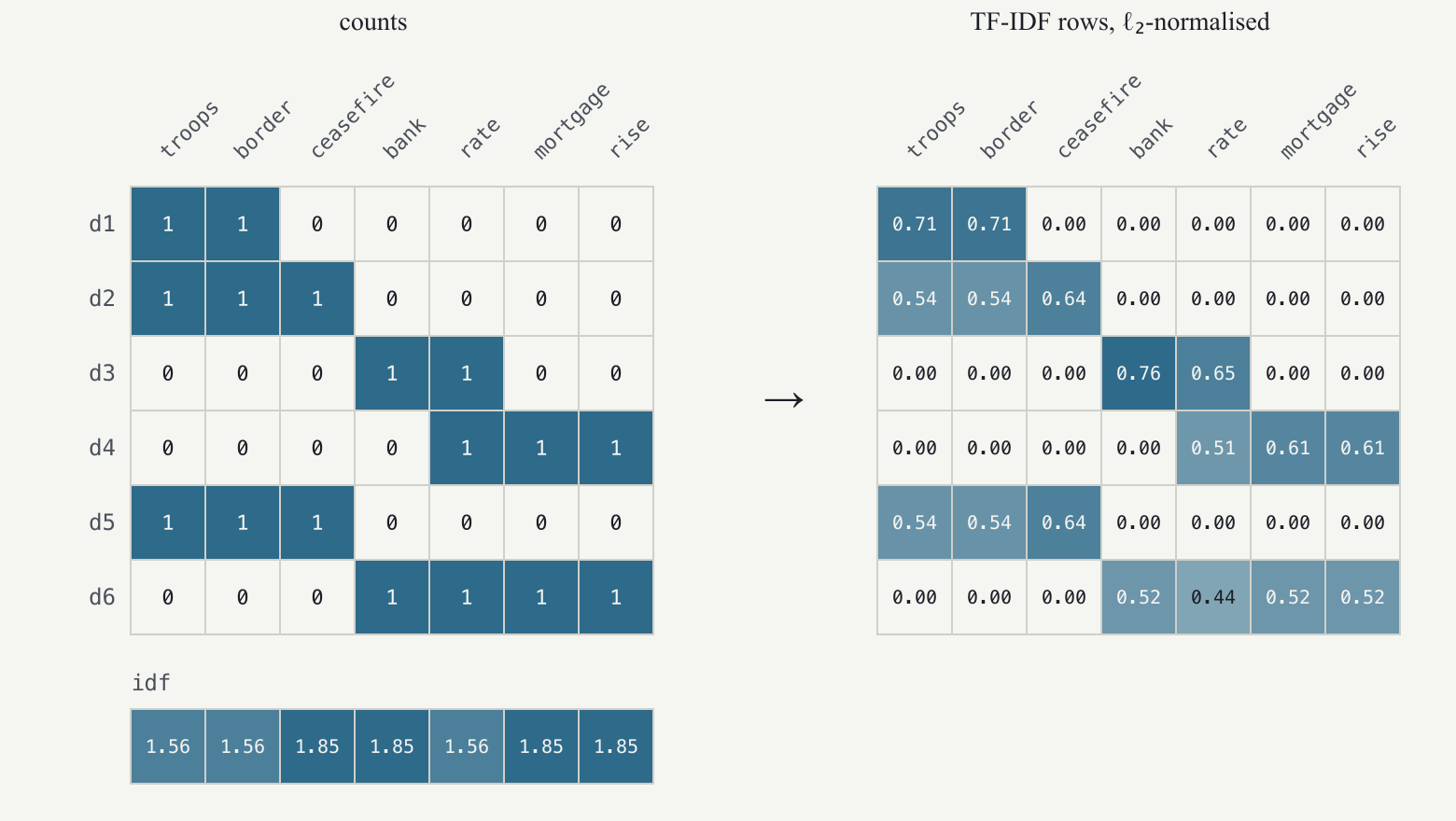
The oldest way to turn a document into numbers is to count its words. Let $p$ count the terms in a fixed vocabulary; a document becomes a row of $p$ counts. A corpus is the collection of documents being analysed. Six tiny “articles”, labelled d1 through d6, and seven retained terms are enough to see the construction:

d1  troops shell border town
d2  ceasefire troops border
d3  bank raises rate
d4  rate rise hits mortgage
d5  troops ceasefire talks border
d6  bank mortgage rate rise

Terms that occur in only one document (shell, town, raises, hits, talks) are dropped in this example—they provide no shared term for connecting documents—leaving troops, border, ceasefire, bank, rate, mortgage, rise. Fix that order before writing any numbers. Document d1 then has row $(1,1,0,0,0,0,0)$: one occurrence of troops, one of border, and none of the other retained terms. Document d3 has row $(0,0,0,1,1,0,0)$. Their first entries refer to the same term even though the documents concern different subjects.

Stacking the six rows creates the count matrix, the left grid of Figure 1. Reading across answers “which retained words does this document use?” Reading down the troops column finds three documents containing that word. A count inside one row and a count of documents down a column answer different questions. The weighting rule below uses both.

2.2 TF‑IDF

TF‑IDF means term frequency–inverse document frequency. Its two factors answer two questions: how often does this document use a term, and how widely does that term occur across documents? Raw counts favour long documents and give common and rare words the same weight per occurrence. We soften the first effect and adjust the second.

2.2.1 Logarithms before the weighting rule

A power repeats multiplication: $2^3=2\times2\times2=8$. A logarithm reverses this question: to what power must a chosen base be raised to produce a given positive number? The natural logarithm, written $\ln$, uses the fixed positive base $e\approx2.71828$. Thus $\ln(e)=1$ and $\ln(1)=0$, because the first and zeroth powers of $e$ are $e$ and 1. The operator $\approx$ means approximately equal. Real-number powers extend this relationship between whole-number powers; we do not need to construct that extension to use a calculator’s log function.

The useful property is that doubling a positive input adds the same amount, $\ln(2)$, to its logarithm. Doubling a count repeatedly therefore adds rather than doubles its contribution. For positive counts 1, 2, 4, and 8, the values of $1+\ln(\text{count})$ are approximately 1.000, 1.693, 2.386, and 3.079. Eight mentions still count more than one, but they do not receive eight times the weight. This is damping.

Let $t$ identify a vocabulary term, $N$ count documents, and $\mathrm{df}(t)$ count the documents containing $t$. For a positive within-document count, define damped term frequency by $\mathrm{tf}=1+\ln(\text{count})$. An absent term gets zero directly; we never ask for $\ln(0)$, which is not defined as a real number. Define inverse document frequency, denoted $\mathrm{idf}(t)$, by

$$\mathrm{idf}(t) = \ln\frac{N + 1}{\mathrm{df}(t) + 1} + 1,$$

Read the formula from inside outward. Add one to both document counts, divide, take the natural logarithm, then add one. The additions inside the fraction are a smoothing convention; the addition outside ensures that a term present in every document still has idf 1. Fewer containing documents make the denominator smaller, the ratio larger, and the idf larger.

There are six documents. Troops appears in three, so its calculation is $1+\ln(7/4)\approx1.56$. Ceasefire appears in two, so its calculation is $1+\ln(7/3)\approx1.85$. Multiply each term’s damped frequency by its idf. In these tiny documents each retained term occurs at most once, so each nonzero damped frequency is 1. Weighting changes how much each present word contributes without inventing a contribution for an absent word.

2.2.2 Turning a weighted row into a unit row

We next remove the row’s overall scale. For a row $a$ with entries $a_t$, the squared Euclidean length is the sum of the squared entries, $\sum_t a_t^2$. The summation sign means add over all vocabulary positions $t$. Squaring means multiplying an entry by itself. The Euclidean length, also called the norm and written $\lVert a\rVert$, is the nonnegative square root of that sum. A square root undoes squaring for a nonnegative result. In symbols,

$$\lVert a\rVert=\sqrt{\sum_t a_t^2}.$$

The double bars denote a vector’s length. Single bars around one scalar will mean its absolute value, or magnitude without sign: $|-2|=2$. A length is nonnegative even when some vector entries are negative.

For d2, only the first three weighted entries are nonzero. Using the unrounded idf values, its length is approximately 2.8770. Dividing each entry by that same length gives approximately $(0.5421,0.5421,0.6421,0,0,0,0)$. Squaring and adding the unrounded normalized entries gives 1. Such a vector is a unit vector. Dividing every entry by one common positive number changes length without changing direction. This is normalization; it leaves the relative proportions of words in the row intact. An all-zero row has length zero and cannot be normalized by division.

Eigen Times builds this representation over 1,093,166 articles and a 50,000‑term vocabulary, keeping terms that occur in at least 20 documents and at most 30% of them. The result has 149 million non‑zero entries out of 55 billion cells—it is 99.7% zeros. Sparse storage keeps only nonzero entries and their positions; dense storage allocates every cell. The algorithms of §5 avoid forming this full matrix densely.

2.3 Cosine similarity

Let $a$ and $b$ be two nonzero rows with the same vocabulary order, and $a_t,b_t$ their entries for term $t$. Their dot product, also called the Euclidean inner product and written $a\cdot b$, multiplies corresponding entries and adds them. For three entries this means $a_1b_1+a_2b_2+a_3b_3$; for a vocabulary it means $\sum_t a_tb_t$. Shared nonzero coordinates can contribute; a product involving an absent coordinate is zero.

The dot product alone grows if we multiply either vector by a large positive number. Cosine similarity, written $\cos(a,b)$, removes this dependence on overall length by dividing by both norms:

$$\cos(a, b) = \frac{a \cdot b}{\lVert a\rVert \, \lVert b\rVert } = \sum_t a_t b_t \quad \text{when } \lVert a\rVert = \lVert b\rVert = 1.$$

A cosine of 1 means the same direction, 0 means perpendicular directions, and $-1$ means opposite directions. In geometric language cosine is the horizontal coordinate of a unit direction measured relative to the first direction; this connects the formula to angles. Its value always lies between −1 and 1. For nonnegative word-count or TF‑IDF rows, negative cosines cannot occur; later centered or embedded vectors can have signed entries. The zero row has no defined cosine because the denominator would be zero.

For d2 compared with itself, the dot product is its first normalized entry squared, plus the second squared, plus the third squared; the remaining products are zero. Normalization made that sum 1. Document d5 has exactly the same retained row, so the same calculation gives 1 for d2 versus d5. For d1 versus d3, every coordinate product is zero: wherever one row has a nonzero retained term, the other has zero. Their dot product, and therefore their cosine, is zero.

In Figure 1, d2 and d5 share troops, border, ceasefire in the same proportions and have cosine 1.0; d1 and d3 share nothing and have cosine 0. Cosine is the similarity used throughout Eigen Times—for clustering a day’s articles into stories, for threading stories into episodes, for finding precedents—so §8 is largely about what values of it mean.

2.4 Embeddings

A TF‑IDF vector knows only which words appear. Two headlines using no shared retained terms have perpendicular, or orthogonal, TF‑IDF rows even if their meanings agree. A sentence embedding is a vector produced by a trained neural network—a numerical model that learns from examples—in which cosine similarity can track meaning beyond vocabulary. Eigen Times uses bge-small-en-v1.5, trained on hundreds of millions of sentence pairs, to turn a headline and lede (opening text: the first 300 characters, at most 96 tokens, or model text units) into 384 numbers. We treat the network as a black box that gives us a vector; everything downstream is linear algebra.

An embedding coordinate need not name a recognizable topic. Meaning is represented by the pattern across coordinates and relationships among vectors. This is why a direction in embedding space will later need evidence from words before we give it a readable name.

These embedding vectors are dense and not centred: their mean—the coordinate-by-coordinate average—has not been subtracted. To see why this matters, consider the synthetic vectors $(1,1,0)$ and $(1,0,1)$. Their dot product is 1 and each has length $\sqrt2$, so their cosine is $1/(\sqrt2\sqrt2)=0.5$. Remove the shared component $(1,0,0)$ from both. The remaining vectors are $(0,1,0)$ and $(0,0,1)$, whose cosine is zero. Normalizing the original vectors would not remove that shared component; subtracting it changes their directions.

News embeddings also share a large common component, and the observed cosine between unrelated articles is around 0.5, not 0. The synthetic calculation demonstrates a mechanism; it does not reproduce that empirical distribution. The observation drives two of the thresholds in §8 and §9.