3 Matrices, pictured

3.1 A matrix times a vector

Let $n$ count document rows and $p$ count their coordinates. Stacking them gives an $n\times p$ matrix $X$: the shape always lists rows before columns. Individual observation vectors will be written as columns when used in projection or outer-product formulas; their transposes supply the rows of a data matrix. A transpose exchanges rows and columns and is marked $\top$. Thus a column $x$ has row form $x^{\top}$.

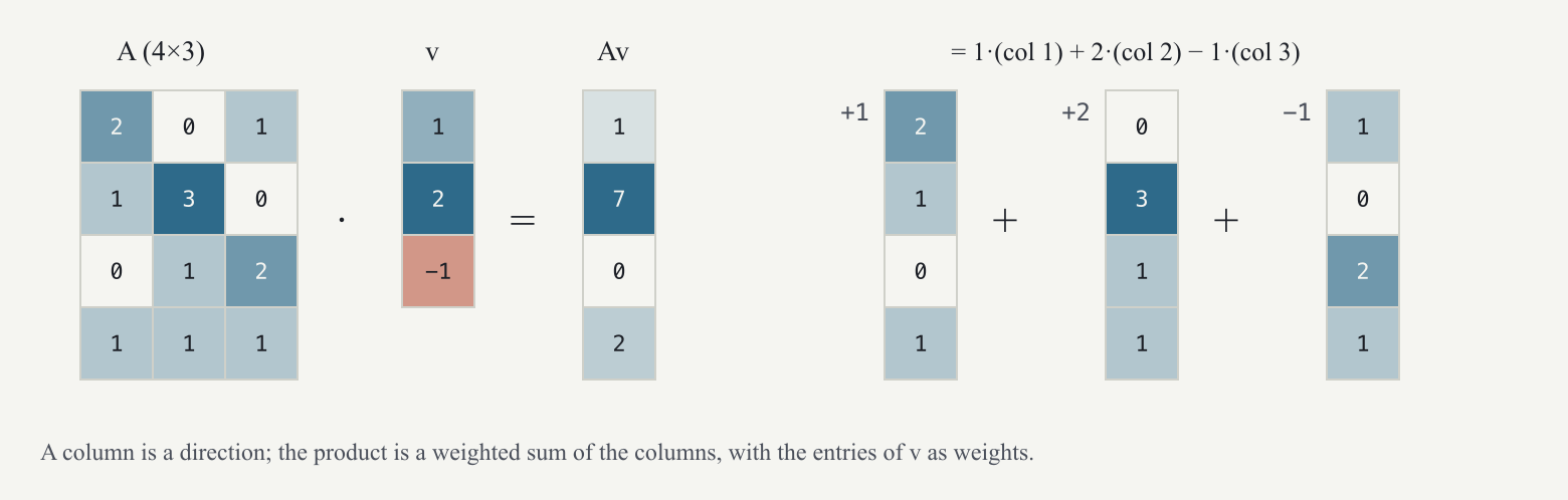
For Figure 2, let $A$ be a $4\times3$ example matrix and $v$ a $3\times1$ column of weights, with entries $v_1$ through $v_3$. Their product $Av$ is a $4\times1$ column. Adjacent mathematical symbols mean multiplication when their shapes permit it.

The actual inputs and result are

$$A=\begin{pmatrix}2&0&1\\1&3&0\\0&1&2\\1&1&1\end{pmatrix},\qquad v=\begin{pmatrix}1\\2\\-1\end{pmatrix},\qquad Av=\begin{pmatrix}1\\7\\0\\2\end{pmatrix}.$$

The second output entry is $1\times1+3\times2+0\times(-1)=7$. Each row of $A$ has three entries and meets all three entries of $v$. This is why the number of columns in the matrix must equal the number of entries in the input column. There are four rows to evaluate, so the output has four entries. A negative weight is allowed: it subtracts a contribution rather than adding one.

The definition of $Av$ is “dot each row of $A$ with $v$”, but the picture to keep is the other one (Figure 2): $Av$ is a weighted sum of the columns of $A$, with the entries of $v$ as the weights. If the columns of $A$ are directions, $Av$ is the point you reach by going $v_1$ of the way along the first, $v_2$ along the second, and so on. That is what “coordinates” will mean in §7: the coordinates of a story are the weights that best rebuild it from the basis directions.

In this example, take the first column once, the second column twice, and subtract the third column once. The second entries combine as $1+2\times3-0=7$, just as in the row calculation. Both descriptions perform the same multiplications; they group them differently. We will use row products to measure coordinates and column combinations to rebuild observations.

3.2 A matrix times a matrix

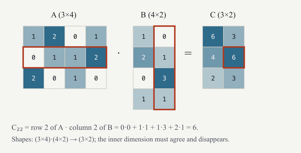
For Figure 3, take a new $3\times4$ example $A$, let $B$ be $4\times2$, and call their product $C=AB$. Indices $i$ and $j$ select a row and column: entry $C_{ij}$ is the dot product of row $i$ of $A$ with column $j$ of $B$. Shapes must agree in the middle: $(3\times4)(4\times2)$ gives $3\times2$. Each column of $B$ is a separate input vector; multiplying by a matrix carries out both matrix–vector calculations together.

Here are the inputs, with the second row and second column providing a short calculation:

$$A=\begin{pmatrix}1&2&0&1\\0&1&1&2\\2&0&1&0\end{pmatrix},\qquad B=\begin{pmatrix}1&0\\2&1\\0&3\\1&1\end{pmatrix}.$$

The entry $C_{22}$ is $0\times0+1\times1+1\times3+2\times1=6$. The four intermediate products correspond to the common inner dimension, 4. The two outer dimensions say that there will be three output rows and two output columns. Matrix multiplication is not entry-by-entry multiplication, and reversing the order need not give the same shape or result.

Two special cases recur. If $X$ has $n$ rows and $p$ columns, $X^{\top}X$ has shape $p\times p$. A row of $X^{\top}$ is a column of $X$, so each output entry compares two columns of $X$ by their dot product. This is called a Gram matrix, and it is the raw material of covariance. In contrast, $XX^{\top}$ compares pairs of observation rows and has shape $n\times n$.

For the other special case, let $k$ count selected, mutually perpendicular unit directions and let $V$ contain them as $p\times1$ columns. Then $XV$ has shape $n\times k$. Entry $(i,j)$ asks how much observation $i$ points along direction $j$. This table contains every document’s coordinates on those directions: the archive projected onto them. We will derive the reconstruction corresponding to those coordinates rather than assuming that taking a projection preserves everything.

3.3 Transpose, symmetry, orthogonality

$A^{\top}$ flips rows and columns. A square matrix has the same number of rows and columns. Call such a matrix $S$; it is symmetric when $S=S^{\top}$. Real symmetric matrices, including covariances, admit a complete set of real, mutually perpendicular eigenvector directions, defined in the next chapter.

3.3.1 Perpendicular directions and what their products say

Two vectors are perpendicular when their dot product is zero. Unit-length perpendicular columns are orthonormal: “ortho” refers to perpendicularity and “normal” to unit length. The identity matrix $I$ has ones on its diagonal and zeros elsewhere; multiplying by it changes nothing. A $p\times k$ matrix $V$ with orthonormal columns satisfies $V^{\top}V=I$, with a $k\times k$ identity. Each diagonal entry in this product is a column’s squared length, so it is 1. Each off-diagonal entry compares two different columns, so it is 0.

Directions are independent when none can be formed as a weighted combination of the others. A basis is an independent collection spanning the space under discussion: its combinations reach every point in that space. The dimension counts the number of basis directions. A matrix’s rank counts the independent directions among its columns, equivalently among its rows. Listing a direction twice does not give us an extra independent direction.

3.3.2 A rotation keeps a whole space; a projection keeps part

If $k=p$, the matrix $V$ is square and orthogonal. It has enough orthonormal columns to describe the whole space. Multiplication by $V$ or $V^{\top}$ rotates or reflects coordinates and preserves lengths and angles. It also satisfies $VV^{\top}=I$, so projecting and rebuilding recovers every input exactly.

If $k<p$, the map $V^{\top}x$ keeps only selected coordinates of an observation column $x$. Rebuilding gives $VV^{\top}x$, its orthogonal projection onto the retained subspace. Now $VV^{\top}$ need not be the identity: the missing directions cannot be recovered merely by changing back to the original number of coordinates.

For the notebook’s example, take $x=(1,2,3)^{\top}$ and let $V$ contain the first two coordinate directions in three dimensions. The superscript $\top$ makes the displayed list a column. Projection gives $(1,2)^{\top}$ and rebuilding gives $(1,2,0)^{\top}$. The squared lengths are $1+4+9=14$ before projection and $1+4=5$ afterward. Nine units of squared length lie in the discarded coordinate. The rectangular matrix obeys $V^{\top}V=I$, but the reconstruction operator is the diagonal matrix with entries 1, 1, 0, not a three-dimensional identity.

A quarter-turn in the retained plane maps $(1,2)^{\top}$ to $(-2,1)^{\top}$. The squared length remains $4+1=5$. This separates two operations that the later pipeline uses for different purposes: retaining a subspace loses information; rotating coordinates within it does not.