A threshold turns a numerical measurement into a decision: link two articles if their similarity reaches a chosen value; highlight an axis if its standardized departure exceeds a chosen size. The measurement and the decision are separate. Cosine supplies a similarity, but mathematics alone does not say which cosine deserves a link.
The thresholds described here use cosines, z-scores, and counts. This chapter shows the empirical distributions used to choose them for the dated Eigen Times corpus. The methods also apply to Eigen Hacks, but these recorded newspaper measurements are not measurements of its technology-community corpus. A changed embedding model, input length, language, or corpus can change the distribution enough to require a fresh assessment.
Start with a graph: a collection of nodes and connections called edges. Here each article is a node. Compare each pair of that day’s article vectors; add an undirected edge when their cosine reaches the chosen threshold. Undirected means that a link from the first article to the second is also a link back.
Next follow links, including indirect links. A path is a sequence of edges joining successive nodes. A connected component is a maximal group joined by paths: no linked node has been left outside it. Each component becomes one story. An isolated article is a singleton, a component of size one.
This rule is called single linkage because one eligible link is enough to join groups. It does not require every pair in a story to meet the threshold. A union–find data structure implements that decision economically: each node begins in its own group; whenever an edge joins two groups, their group records are merged. It is a bookkeeping method for the same connected components, not an additional similarity rule.
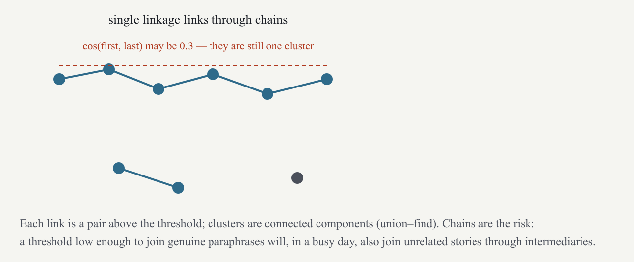
The notebooks show the resulting chaining with four synthetic unit directions at 0, 30, 60, and 90 degrees. Adjacent directions have cosine about 0.866, so a threshold of 0.72 joins all four through a chain. The endpoints have cosine zero but still belong to one component. At 0.9, none of those synthetic pairs link. Figure 13 illustrates the danger: on a busy day, intermediate similarities can connect unrelated endpoints and let one chain absorb much of the news.
Figure 14 examines the cosines of article pairs on five busy days (12 September 2001, 16 September 2008, 24 June 2016, 12 March 2020, 24 February 2022), split by whether the two ended up in the same story. A distribution describes how values are spread across possible sizes. A histogram groups them into intervals, or bins, and counts values in each interval. The sample’s median is its middle value; its 99th percentile is a value at or below which about 99% of observations lie. The figure scales each histogram to its own highest bin, so equal displayed heights do not mean equal pair counts or equal probabilities. These are descriptive same-story labels from the grouping, not an independent human-labeled test set. In embedding space, pairs from different stories have median cosine 0.49 and a 99th percentile of 0.67—confirming that unrelated news embeddings sit around 0.5, not 0—while pairs from the same story have median 0.65 and a long tail toward 1. The two distributions overlap, as they must for anything less than a perfect representation, but the crossover is narrow.
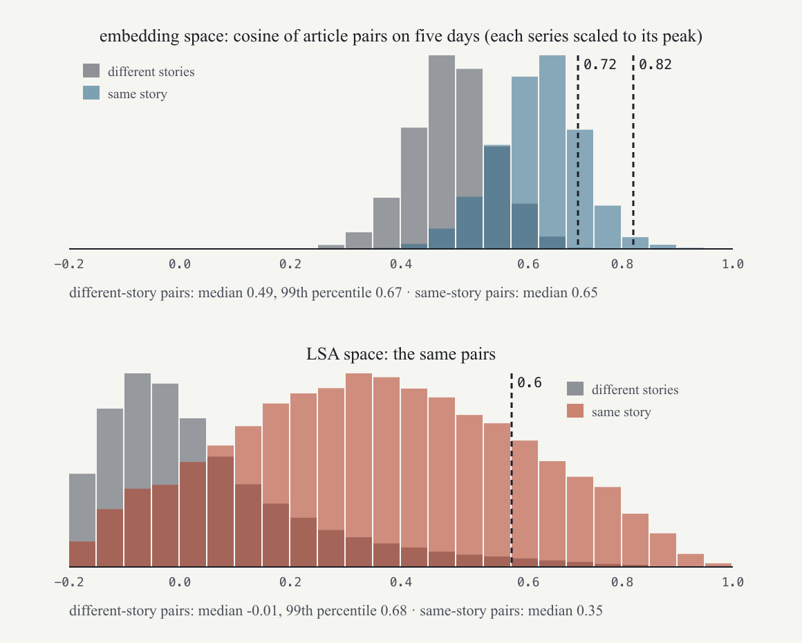
Choosing a threshold balances two failures. Lowering it adds edges, which can join distinct events through chains. Raising it removes edges, which can split one event into several components; this is fragmentation. Figure 15 shows the search for a useful balance on 24 February 2022, the day Russia invaded Ukraine. At 0.6, one chain contains 143 of the day’s 152 articles—most of the day has become one “story”. At 0.66 the chain still holds 104. At 0.72 the largest cluster is the 62‑article invasion story, the intended grouping identified during inspection, with 67 singletons (features, comment, unrelated items). At 0.78 the invasion story has fragmented to 34 articles; at 0.82 no cluster is larger than 8; at 0.9 only one linked pair remains: 151 components, the largest of size 2, and 150 singletons among 152 articles. These are the counts in the frozen aggregate fixture; the earlier wording that nothing linked was incorrect. The deployed threshold is 0.72. The sweep shows the effect of this choice on that day’s graph; it does not prove an optimal threshold for every possible day. The original choice had been 0.82 (a number appropriate for a larger embedding model with longer inputs); the first look at the data—“Day of terror” on 12 September 2001 rendered as a three‑article story—showed it was wrong, and the sweep in Figure 15 replaced it.
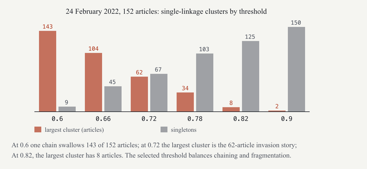
The lower panel of Figure 14 explains why the LSA space needs a different threshold. LSA coordinates are projections onto the 60 leading right singular directions of the term matrix; articles about the same event share vocabulary but in a 60‑dimensional summary their cosines spread from 0 to 1 (median 0.35), and unrelated articles sit around 0 (median ). The distributions are wider and cross lower, and the threshold that reproduces sensible stories is 0.6. The same numerical threshold therefore has a different meaning in the two representations. Their coordinate systems and similarity distributions differ. This is one reason the deployed newspaper clusters in embedding space and uses the LSA basis only for measurement. The notebooks can recompute the histogram scaling and proportions from frozen aggregate counts; they cannot recreate historical cluster assignments without the original article vectors.
An episode is a chain of related stories across days. First summarize each story by its centroid: average its member embedding vectors, then use that mean’s direction in the cosine comparison. Averaging is done coordinate by coordinate. A zero mean has no direction, so an implementation must handle that case explicitly rather than calculate an undefined cosine.
In this subsection indexes calendar days, distinct from the earlier term index. To thread a story on day , compare its centroid with each story centroid on day . Keep the greatest cosine, the best match. If it reaches 0.9, continue that previous story’s episode; otherwise start a new episode. This is a best-previous-story rule, not a one-to-one assignment between all stories on the two days. Several current stories can independently select the same previous episode.
The threshold acts after the maximum is found. In the notebook’s synthetic two-story example, one current centroid has best similarity 0.92 and continues; the other fails the 0.9 threshold and starts a new episode. A best match always exists when there are eligible nonzero previous vectors, but it need not be a good match. Figure 16 shows, for 678 stories over eight day-pairs, each best previous-day cosine. With raw embeddings the median is 0.66 because unrelated news shares a common component. Reported continuations above the strict threshold include “Battle for Kyiv” after “Putin invasion deepens” (0.92), the Hamas attack’s death toll two days running (0.90), and Brexit voters’ portraits (0.93). In late February 2022, 21 of 1,077 stories continued an episode, and the longest, the invasion, ran fourteen days from 18 February to 3 March.
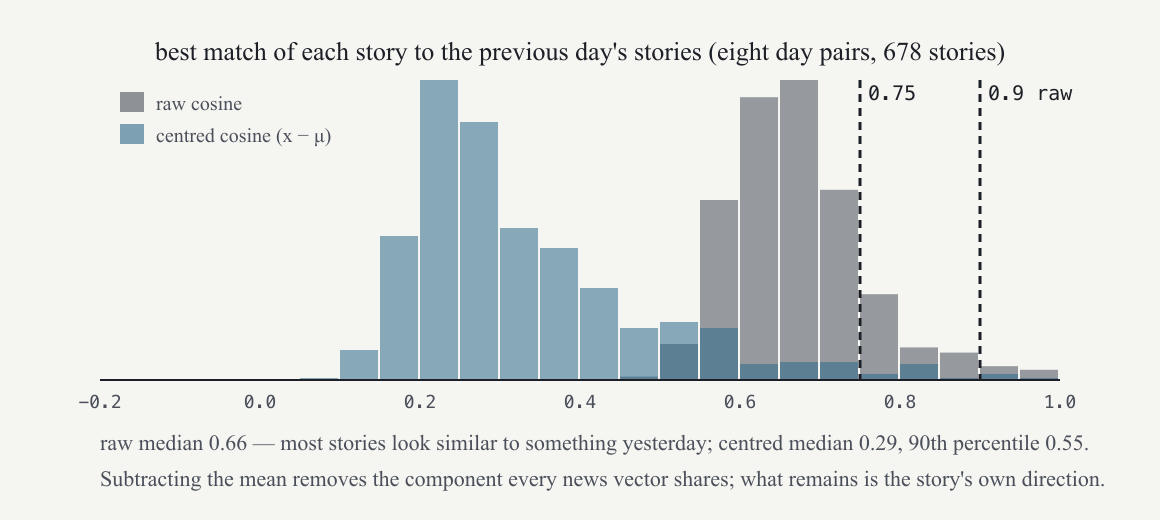
Subtracting the mean first removes the common component and lowers the median to 0.29, with a sparser region around 0.55–0.75. A centred threshold near 0.75 is a candidate for separate evaluation, not a direct replacement proved by the figure. It would still miss the cited Crimea continuation at 0.69; lowering it enough to include that pair could also admit the unrelated New Zealand protest and abortion pair at 0.70. To assess this tradeoff, first obtain judgments of which candidate links really are continuations. Precision is the number of correct accepted links divided by all accepted links. Recall is the number of correct accepted links divided by all true continuations in the evaluated set. If no link is accepted, precision has a zero denominator; if the evaluated set has no true links, recall does too. Those cases need explicit reporting conventions.
The notebooks supply five labeled synthetic candidates: three true links at 0.92, 0.90, and 0.93, a false link at 0.70, and a true link at 0.69. A 0.9 threshold accepts three correct links: precision is and recall is . Lowering it to 0.69 recovers all four true links but also accepts the false one: precision becomes and recall . Those labels are teaching inputs, not a new evaluation of the historical stories. The strict raw rule aims to favor precision. An episode is a thread, not a day: “episode day 7” counts from the chain’s beginning, and an archetype’s canon counts episodes rather than repeated days.
A precedent is an earlier candidate presented for comparison, not proof that history will repeat. The search has an eligibility stage and a ranking stage.
First retain only stories earlier than the query story and having the same dominant axis. This prevents future stories from entering a historical comparison and makes the archetype part of the search definition. Then compare named-coordinate vectors by cosine. Among stories from the same episode, keep the strongest match; finally take the five strongest remaining matches, or fewer if fewer are eligible. The distinct-episode restriction avoids filling the list with five days of the same event.
No similarity threshold is required to return the nearest eligible candidates. This is a ranking: the largest scores come first. A ranking can still return weak matches if all eligible candidates are weak. Printing the cosine beside each precedent lets the reader assess that distinction: recorded examples include 0.97 for the same week’s build-up briefing and 0.93 for Crimea in 2014. A shared dominant axis or a large cosine establishes resemblance in this representation, not a causal relationship between the events.