7 Measuring a story

7.1 Projection, reconstruction, residual

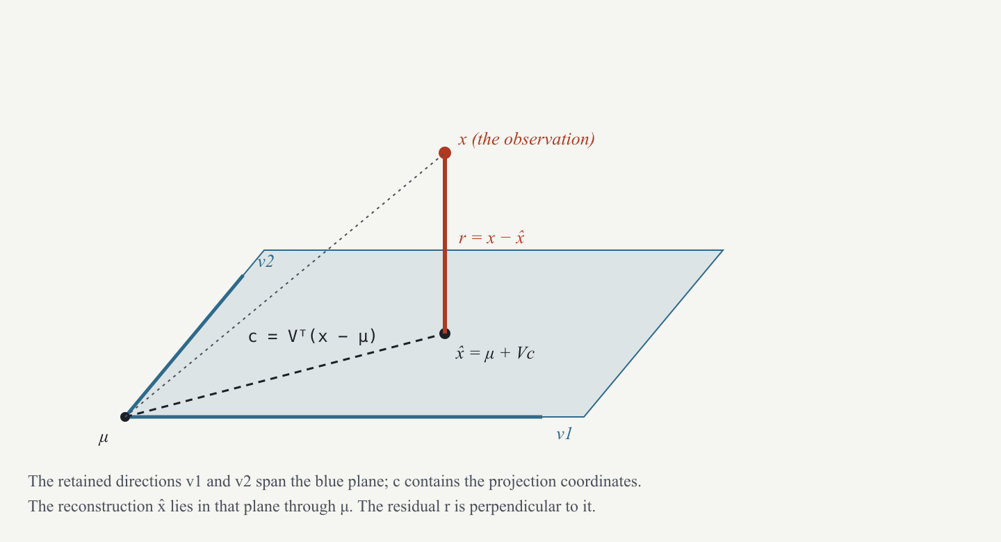
The question is now about one observation: how much of it can the retained directions reconstruct, and what do they leave out? Here an observation is an article, or a representative vector chosen for a story. It is already a numerical vector; we are not yet assigning it a claim about historical novelty.

Let $d$ count its original coordinates and $k$ count retained directions. Write $x$ for the $d\times1$ observation column and $\mu$ for the $d\times1$ fitted article mean. The $d\times k$ matrix $V$ contains the retained raw directions as columns. They are orthonormal: each has length one and different columns have dot product zero. The following steps have different jobs.

7.1.1 First find coordinates, then reconstruct

Subtract the reference point. The centred column $x-\mu$ is the displacement from the fitted mean. Projection concerns this displacement, so the mean must be removed before measuring coordinates.

Measure along each retained direction. Define the $k\times1$ coordinate column $c$. Entry $c_j$, with $j=1,\ldots,k$, is the dot product with retained direction $j$. Stacking those dot products is matrix multiplication:

$$c=V^{\top}(x-\mu).$$

Rebuild what those coordinates describe. Multiplying by $V$ takes the weighted sum of the retained directions. Adding the mean puts the result back in the original coordinate system. Call this $d\times1$ reconstruction $\hat x$; the hat marks an approximation:

$$\hat x=\mu+Vc.$$

Subtract the reconstruction from the observation. The $d\times1$ difference $r$ is the residual: what remains after the attempted reconstruction. The word names a difference vector, not its length and not its probability:

$$r=x-\hat x.$$

For a complete synthetic example, retain the first two coordinate directions in three dimensions. Take $x=(2,1,3)^{\top}$ and $\mu=(0,0,0)^{\top}$. Then

$$V=\begin{pmatrix}1&0\\0&1\\0&0\end{pmatrix},\qquad c=\begin{pmatrix}2\\1\end{pmatrix},\qquad \hat x=\begin{pmatrix}2\\1\\0\end{pmatrix},\qquad r=\begin{pmatrix}0\\0\\3\end{pmatrix}.$$

The first coordinate survives unchanged, the second survives unchanged, and the third is absent from the retained plane. Subtraction reveals that absence explicitly: $3-0=3$ in the last residual entry.

7.1.2 Why this is the nearest reconstruction

An orthogonal projection keeps the component in the chosen subspace and leaves a residual perpendicular to it. Here this can be checked by taking its coordinates again. Since $V^{\top}V=I$, where $I$ is the $k\times k$ identity,

$$V^{\top}r=V^{\top}(x-\mu)-V^{\top}Vc=c-c=0.$$

Thus every retained direction has zero dot product with the residual. This is also why the reconstruction is a least-squares one. Any change to the reconstructed point within the retained subspace adds another perpendicular component to the error. Its squared length adds to the existing residual squared length, so it cannot improve the fit. No differentiation is needed for this geometric argument.

Recall the two distinct operations in a length calculation. Squaring entries and adding them gives squared length; taking its square root gives length. For our residual,

$$\lVert r\rVert^2=0^2+0^2+3^2=9,\qquad \lVert r\rVert=\sqrt9=3.$$

The centred observation has squared length $2^2+1^2+3^2=14$. The retained part has squared length $2^2+1^2=5$. The Pythagorean identity reads $14=5+9$: retained variation and residual variation account for the whole squared length. We use squared lengths below because perpendicular contributions add in this way. The ordinary lengths do not add: $\sqrt{14}$ is not $\sqrt5+3$.

7.2 T² and Q

We need two different comparisons. One asks how far the story lies along the retained directions, taking each direction’s usual spread into account. The other asks how much of the story lies outside those directions. A statistic is a numerical summary calculated from data; calling something a statistic does not by itself assign a probability to it.

7.2.1 Compare a coordinate with its usual spread

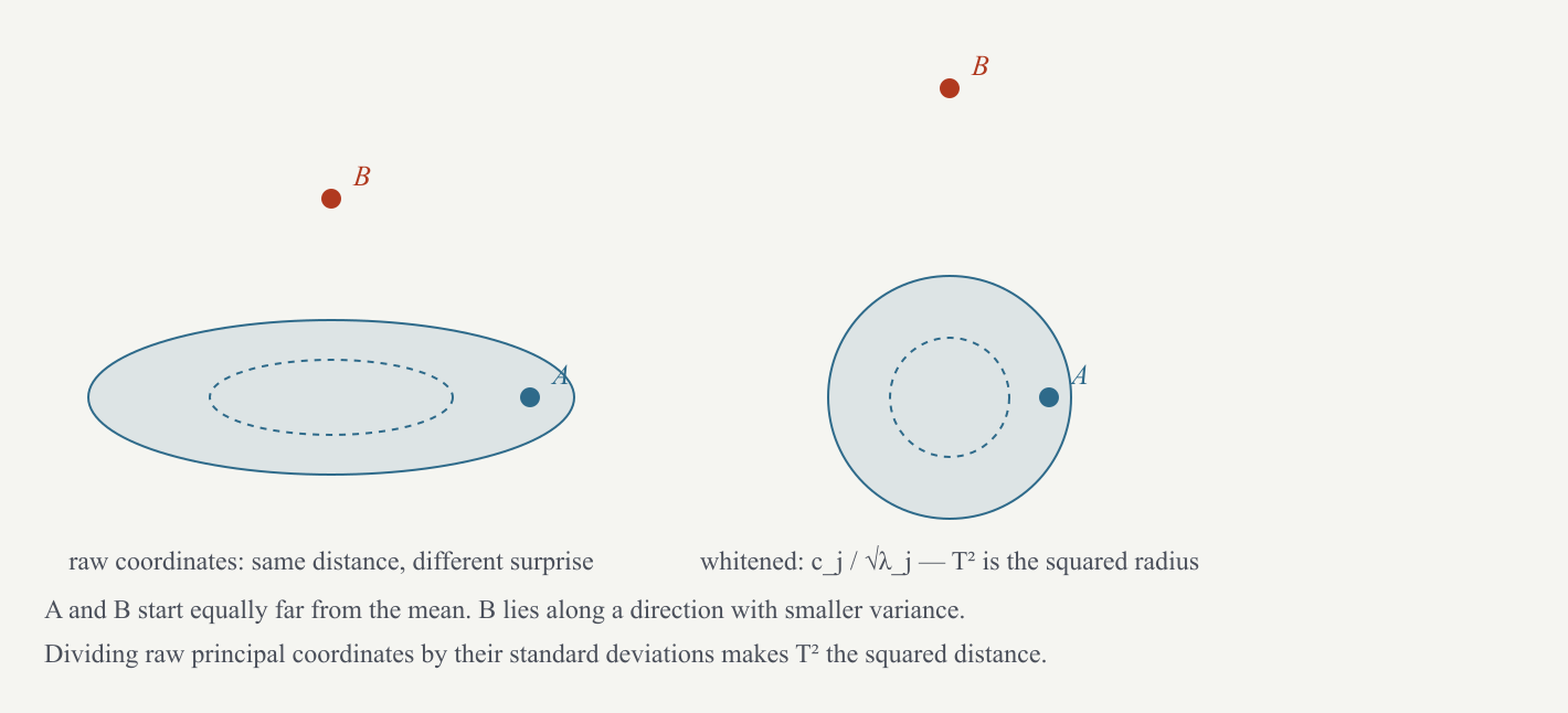
Recall that variance is an average squared deviation from a mean, and standard deviation is its nonnegative square root. Raw coordinate $j$ has fitted mean zero and variance $\lambda_j$. For this calculation retain only positive eigenvalues, so dividing by $\sqrt{\lambda_j}$ is possible. The quotient $c_j/\sqrt{\lambda_j}$ expresses the coordinate in units of its own standard deviation. A displacement of two units is ordinary on an axis whose usual spread is two, but larger relative to an axis whose usual spread is one.

A z-score subtracts a reference mean and divides by a positive reference standard deviation. The mean subtraction has already happened for the raw coordinates. Their variances can differ, but their fitted cross-covariances are zero. Dividing each by its own standard deviation therefore gives whitened coordinates: unit variance in every direction and zero cross-covariances under that same fitted reference.

Define $T^2$, Hotelling’s squared covariance-adjusted distance, by squaring these standardized coordinates and adding. Here $T^2$ is the statistic’s name, not the square of the TF‑IDF matrix $T$. With $j=1,\ldots,k$,

$$T^2=\sum_j\left(\frac{c_j}{\sqrt{\lambda_j}}\right)^2 =\sum_j\frac{c_j^2}{\lambda_j}.$$

Our synthetic story has $c=(2,1)^{\top}$. Suppose the fitted raw variances are $4$ and $1$, hence standard deviations $2$ and $1$. Its standardized coordinates are $(2/2,1/1)^{\top}=(1,1)^{\top}$. Squaring and adding gives

$$T^2=1^2+1^2=2.$$

Both retained coordinates are one reference standard deviation from their means, although their original sizes differ.

For compact matrix notation let $\Lambda$ be the $k\times k$ diagonal matrix of those positive raw eigenvalues. A superscript $-1$ denotes an inverse, the operation undoing multiplication by an invertible matrix. For a diagonal matrix, inversion replaces each nonzero diagonal entry by its reciprocal. Consequently $\Lambda^{-1}$ first divides coordinate $j$ by $\lambda_j$; the dot product with $c$ then multiplies by $c_j$ again and adds:

$$T^2=c^{\top}\Lambda^{-1}c.$$

7.2.2 Measure the part outside the retained space

Define $Q$ to be residual squared length:

$$Q=\lVert r\rVert^2.$$

For the same story, $Q=9$. This is a different measurement from $T^2=2$. A point can be far along a retained direction and have no residual at all; another can lie close to the mean within the retained directions but have a substantial perpendicular residual. A residual can contain discarded familiar variation as well as genuinely new material. Neither statistic alone proves that an event is unprecedented.

Figure 12 shows why reference spreads matter: equal Euclidean distances can have different covariance-adjusted distances. With 60 fitted positive directions, the fitted average of $T^2$ under the matching covariance weights is 60. To see why, average each term $c_j^2/\lambda_j$: the numerator’s fitted average is precisely $\lambda_j$, so every term contributes one. A value of 400 is much larger than that fitted average. This arithmetic does not yet provide the probability of reaching 400; that would require a justified probability model or a separately assessed reference distribution.

7.2.3 Keep the covariance when changing coordinates

The calculation uses raw eigen-coordinates before the naming rotation. The rotation changes the coordinate descriptions without changing the retained point. Recall the $k\times k$ orthogonal naming rotation $R$. In the named coordinate column $y=R^{\top}c$, define the covariance $\Gamma=R^{\top}\Lambda R$. Its off-diagonal entries need not be zero: named coordinates can vary together even though the raw eigen-coordinates did not.

To measure the same distance in this new coordinate system, use its full covariance:

$$T^2=y^{\top}\Gamma^{-1}y.$$

The inverse now adjusts for both different spreads and shared movement between coordinates. Reusing the old diagonal eigenvalues would attach old scales to new directions. Dividing by the named coordinates’ own variances is also insufficient when their covariances are nonzero. That operation is marginal standardization: it gives each coordinate unit variance separately but leaves correlations. Full whitening removes cross-covariances as well. The notebooks rotate the synthetic story and verify that the full calculation stays unchanged while the diagonal shortcut generally changes it.

The implementation sums $c_j^2/\lambda_j$ only for positive raw eigenvalues and contributes zero otherwise. This is an explicit handling rule for zero-variance directions, not permission to divide by zero. The inverse formulas above assume positive retained eigenvalues.

7.2.4 Turn residual size into a share

The two statistics originated in monitoring variation against a principal-component reference model. For browsing, it is also useful to ask what share of a centred observation remains outside the retained subspace. Let $\nu$ (Greek nu) denote this novelty ratio. When $x\ne\mu$, meaning the observation differs from the fitted mean, define

$$\nu=\frac{Q}{\lVert x-\mu\rVert^2}.$$

The denominator counts all centred squared length; the numerator counts only the residual part. In our example, $\nu=9/14\approx0.643$. About 64.3% of this observation’s squared length lies outside the retained plane. That is a statement about this representation, not a 64.3% probability of a historically new event.

Orthogonality makes the denominator the sum of retained and residual squared lengths, both nonnegative. The ratio therefore lies between zero and one. Zero means the centred vector is fully represented; one means it lies perpendicular to the retained subspace. At $x=\mu$, both numerator and denominator are zero, so the ratio is undefined. The implementation returns zero in that case as a software convention. This geometric use of “energy” means squared length; the attention score below uses the same ordinary word for a different quantity.

7.2.5 Average measurements in the order intended

These equations describe one vector. The site’s stored story statistics are means of the member articles’ $T^2$, $Q$, and $\nu$ values. The order matters: measure every member, then average the measurements. Measuring the mean embedding answers a different question.

For example, two member coordinate columns $(2,0)^{\top}$ and $(-2,0)^{\top}$ under variances $(4,1)$ each have $T^2=4/4=1$, so their mean statistic is one. Their mean coordinate column is zero, whose $T^2$ is zero. Averaging first cancels their opposite departures. Squared distances and ratios generally do not commute with averaging; that is why an article statistic, an average article statistic, and a centroid statistic must be kept distinct.

7.3 Dominant axis, spectrum, profile

These three objects answer questions at three different levels. The dominant axis selects a story’s label. The spectrum combines the day’s stories. A profile describes the stories usually carrying one label.

7.3.1 Select a label using comparable signed scores

For story $s$, let $y_s$ be its $k\times1$ named-coordinate column, with entry $y_{sj}$ on axis $j$. Here $s$ identifies a story. The separate notation $s_j>0$ denotes the empirical standard deviation of named coordinate $j$ across stories in the profile window: the latest ten years of loaded data. This is a reference scale, estimated separately from the raw eigenvalue $\lambda_j$. The implementation replaces scales smaller than $10^{-6}$ by that positive floor to avoid division by zero or an extremely small denominator.

Divide each named coordinate by its reference scale. The dominant archetype is the axis with the largest signed result. The notation $\arg\max_j$ means “return the index attaining the largest value”, whereas $\max_j$ would return the value itself. Thus the rule is $\arg\max_j y_{sj}/s_j$.

Take the notebook’s synthetic story $(2,1)^{\top}$ and scales $(2,0.5)$. The scores are $2/2=1$ and $1/0.5=2$, so the second axis wins despite its smaller raw coordinate. For a second story $(-1,-0.1)^{\top}$, the scores are $-0.5$ and $-0.2$. The second wins again because $-0.2$ is larger. Taking absolute values would change that decision. This particular rule does not subtract an empirical axis mean, so it is scale division rather than a general mean-subtracted z-score.

One possible “mixed” heuristic compares the positive top score $a_1$ with the runner-up $a_2$. Their relative gap is $(a_1-a_2)/a_1$; the denominator is the top score. A rule declaring a mixture when that gap is at most $0.20$ would accept scores $1$ and $0.85$, whose gap is $0.15$. This is an illustrative rule retained from the original explanation, not a rule implemented by the current site.

7.3.2 Combine stories into a daily spectrum

A simple average gives every story equal influence. A weighted mean first multiplies each value by its nonnegative weight, adds those products, and divides by the positive total weight. Division by the total makes the result an average rather than a total that grows automatically when more stories are present.

Let $\varepsilon_s$ denote story $s$’s attention weight, called story energy in the site:

$$\varepsilon_s=\text{distinct sources}\times\ln(1+\text{article count}).$$

The natural logarithm grows slowly; adding one makes the argument positive even for a zero count. This weight uses source and article counts. It is distinct from article fit weights, eigenvalues, and vector squared length.

For one chosen day, let $\bar y_{\mathrm{day}}$ be its $k\times1$ spectrum column. The bar indicates averaging, and the sum includes that day’s stories only:

$$\bar y_{\mathrm{day}}=\frac{\sum_s\varepsilon_s y_s}{\sum_s\varepsilon_s}.$$

The notebooks use three synthetic story rows $(2,1)$, $(-1,-0.1)$, and $(0.5,3)$, with source counts $2,1,3$ and article counts $3,1,5$. Their attention weights are $2\ln4\approx2.773$, $\ln2\approx0.693$, and $3\ln6\approx5.375$. For the first spectrum coordinate, multiply $2,-1,0.5$ by those weights, add, and divide by their sum. Repeating for the second coordinate gives approximately $(0.853,2.130)$. The more heavily weighted third story pulls the mixture towards its second coordinate; no new direction has been fitted in this averaging step.

7.3.3 Compare a day, or compare a story

The era statistics are each spectrum coordinate’s mean and standard deviation over all loaded day spectra. The algorithm named after Welford updates three running summaries: how many values have arrived, their current mean, and the sum of squared deviations from that current mean. It adjusts the deviation sum when the mean changes; simply squaring deviations from an outdated mean would give the wrong answer. The statistical-threshold chapter walks through its calculation.

Each spectrum z-score subtracts the coordinate’s era mean and divides by its positive era standard deviation. The front page highlights values beyond $\pm2$ (plus or minus two) and lists values below $-2$ under Silence. These are comparisons with all loaded data, including dates later than some selected historical dates. They are not historical forecasts computed using only the past available at the time.

An archetype’s profile uses a different reference set: the stories it dominates in the profile window. For each named coordinate, it records a mean and standard deviation among those stories. Same as always combines strong positive profile and story signals with agreement within one profile standard deviation; agreement alone is insufficient. Different this time lists departures exceeding 1.5 profile standard deviations. The symbol $\sigma$ in these descriptions is shorthand for the relevant reference standard deviation, not an SVD singular value. A zero reference deviation needs an explicit fallback before any z-score can be computed. Always identify the reference population before interpreting a standardized score.