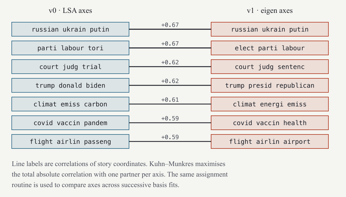
Suppose several old axes each resemble several new axes. Picking the best match for one axis can consume the only good match available to another. We need to consider the whole set of pairings together.
An assignment problem chooses a one-to-one pairing: each old axis receives one new axis, and no new axis is reused. Its objective is to maximize the sum of the chosen similarities. For a small synthetic example, the notebook uses this table; rows name old axes and columns name new axes:
| new A | new B | new C | |
|---|---|---|---|
| old A | 0.90 | 0.80 | 0.10 |
| old B | 0.85 | 0.20 | 0.10 |
| old C | 0.10 | 0.10 | 0.95 |
Taking old A’s strongest match first selects new A at 0.90. If old B then takes new B and old C takes new C, the total is . Swapping the first two matches gives , a larger total. The slightly weaker choice for old A permits a much stronger one for old B. This is why a greedy procedure, choosing the best currently available local option, need not solve the global assignment.
The Hungarian algorithm, also called Kuhn–Munkres, solves the assignment problem without trying every possible permutation. It runs in polynomial time: its work grows no faster than a fixed power of the problem size. The numerical routines implement that search; the similarity table and one-to-one constraint define what it is solving. For nightly comparisons in the same feature space, table entries are absolute eigenvector cosines. Signs are then oriented to agree.
A raw dot product requires matching coordinate meanings and dimensions. The notation means lists of real-number coordinates. A 50,000-term direction and a 384-coordinate embedding direction live in and respectively. Their entries cannot be multiplied pairwise to obtain a meaningful cosine.
Instead ask both directions about the same stories in the same order. Each direction yields one score per story. Those two score columns now have matching observation positions, regardless of the different spaces that produced them.
Compare the score columns using correlation: their covariance divided by their positive standard deviations. Operationally, subtract each column’s own mean, take the dot product of the centred columns, and divide by their lengths. This is the cosine of the centred score columns; the common averaging denominators cancel. Positive correlation means above-mean scores tend to occur on the same stories, negative correlation means they tend to occur on opposite stories, and a constant column has no defined correlation because its centred length is zero.
For intuition, the notebook pairs scores with an identical score column produced in the other space. Their shared ordering and departures give correlation one. Reversing a nonconstant centred column’s sign reverses the correlation. Using these score comparisons as table entries lets assignment match across representations without pretending their original coordinate systems are the same.
The reported study compared scores on the same 100,000 stories. Figure 17 shows selected matches: Ukraine with Ukraine at 0.67 and courts with courts at 0.62; the reported comparisons also include the EU at 0.57. Those are dated empirical associations. The notebook’s small synthetic score table teaches the calculation without re-estimating unavailable archive measurements.
Why should yesterday’s directions resemble today’s at all? One reason is that adding a modest amount of data to a large fixed reference often changes its covariance only a little. A second condition is essential: the direction must be separated from competing directions. If two eigenvalues are equal, rotating their eigenvectors inside their common plane changes the axes without changing the covariance. Near equality can therefore make individual axes sensitive to small changes.
A perturbation is the difference between the new and old matrices. Let be this covariance change, with the same shape as each covariance. Its spectral norm, written , is the greatest output length produces from any unit input. The subscript denotes the Euclidean-length operator norm; it does not mean that all matrix entries have been squared and summed. Define the scalar as the size of the perturbation.
A simple eigenvalue has a one-dimensional eigenspace, so its unit eigenvector is determined up to sign. Consider a matched simple old eigenvalue and a new eigenvalue. Define the positive separation by comparing that new eigenvalue with every other old eigenvalue and taking the smallest distance. This precise comparison is part of the hypothesis. An arbitrary gap taken from a nearby pair of values cannot be substituted without further assumptions.
After matching the signs, let be the acute angle between the two unit eigenvectors. Its sine, , is the length of the component of one direction perpendicular to the other. It is zero when the lines agree and increases towards one as they become perpendicular. The Davis–Kahan bound in this setting is
The inequality gives an upper bound, not a prediction of the exact turn. A smaller covariance change lowers the bound; a smaller separation raises it. If the right-hand side exceeds one, the inequality gives no useful improvement over the fact that a sine is at most one.
The notebook starts with covariance diagonal entries and , then adds to both off-diagonal entries. The perturbation norm is and the specified separation is slightly greater than , so the bound is about . The notebook calculates both the actual turning sine and the bound and checks the inequality. It also rotates a two-direction basis within a fixed plane: individual columns change while the projection onto the plane remains identical. This explains why nearly degenerate groups call for subspace comparisons.
If the added day’s total weight and observation lengths stay bounded while accumulated weight grows in proportion to an observation count , the one-step covariance change can be . This big-O notation means bounded by a constant times under the stated assumptions. Larger accumulated weight then dilutes a bounded new contribution. The statement concerns an individual update. It does not prove that an evolving sequence of news bases converges forever, particularly when the data distribution or weighting policy changes.
Two continuity procedures address different remaining freedoms. Procrustes alignment rotates or reflects a matched group to minimize its total squared difference from the preceding group; it aligns coordinate frames without asserting that the underlying subspace never changed. Warm-starting begins the new varimax optimization at the preceding rotation instead of a fresh starting point. Both can aid continuity, but neither overrides a substantial data change or a vanishing eigengap.