11 Streaming the computation

The first edition of Eigen Times was fitted on 1.09 million articles, and its code could afford to hold what it needed: every article’s embedding and coordinates while the axes were oriented, and the whole document–term matrix while the axes were named. The second edition ingested the New York Times archive back to 1851 and multiplied the corpus by fifteen, to 16.5 million articles. The first attempt to fit it was killed by the operating system at about forty gigabytes. What follows is the arithmetic that let the same computation run in a fraction of a gigabyte—not a bigger machine, but a change of shape. The principle is one sentence: every quantity the fit needs is a sum over documents, and a sum can be taken in blocks.

11.1 Weights that balance the days

Before the sums, the weights. By article count the modern era dominates the archive—the Guardian alone publishes about as many articles a day as the Times index ever recorded—while by the calendar it is fifteen per cent of 175 years. Let $i$ index articles and $\tau$ a calendar day. Write $\tau(i)$ for article $i$’s day and $n_\tau>0$ for the number of eligible articles on that day. The second edition assigns article $i$ the inverse-count weight $w_i$. A sum constrained by $\tau(i)=\tau$ includes only articles from the chosen day:

$$w_i = 1 / n_{\tau(i)}, \qquad \sum_{\tau(i) = \tau} w_i = 1,$$

Every populated day therefore contributes one unit to the fit: a day in 1887 with 40 index entries and a day in 2024 with 900 articles count the same. The arithmetic is $40(1/40)=1$ and $900(1/900)=1$. An article from the smaller day has greater individual weight, while both days have equal total influence.

The notebooks make this distinction visible using a synthetic coordinate that is zero for each of the 40 first-day articles and one for each of the 900 second-day articles. Its article-weighted mean is $900/940\approx0.957$. Its day-balanced mean is $(1\times0+1\times1)/(1+1)=0.5$. Neither is an arithmetic error: they answer different questions about what counts as one unit of influence. Total weight $Z$ is the number of represented days, 63,270. The covariance formulas retain their shapes; the diagonal entries of $W$ change. For term-space fitting, let $\mu_{T,w}$ be the $p\times1$ TF‑IDF mean under these same article weights. Let $W^{1/2}$ be the diagonal matrix of the nonnegative square roots of the article weights. With $T$ of shape $N\times p$ and $\mathbf1$ of length $N$, the balanced LSA fit decomposes $W^{1/2}(T-\mathbf1\mu_{T,w}^{\top})$. Its mean is distinct from the unweighted naming mean $\mu_T$ below.

Why multiply centred rows by square-root weights? The covariance calculation subsequently multiplies a row by its transpose. The two factors each contribute $\sqrt{w_i}$, whose product is $w_i$. Using the full weight on both sides instead would produce $w_i^2$ and answer a different weighting question. Weighting, centering, and normalization each have a separate role; none can be omitted merely because the matrix shapes still match.

11.2 Sums over blocks

Split the article rows into disjoint blocks indexed by $b=1,2,\ldots$. In Eigen Times, a block is one source’s articles for one month; there are about three thousand. The notation $i\in b$ means article row $i$ belongs to block $b$. Let $g$ be any fixed rule converting a row $x_i$ into a scalar, vector, or matrix contribution of the same shape for every row. Then

$$\sum_i g(x_i)=\sum_b\sum_{i\in b}g(x_i).$$

Read the inner sum first: calculate the contributions from articles in one block and add them. The outer sum adds the resulting block totals. Every article must appear in exactly one block; missing or duplicated rows would change the answer. Once a block’s contribution has been added, its article rows can be discarded from memory. Here the function $g$ is unrelated to the eigengap scalar in §10.

For covariance the contributions are already known: an article adds its weight to $Z$, its weighted coordinate column to $m$, and its weighted outer-product matrix to $M$. Each block produces a scalar, a $d\times1$ column, and a $d\times d$ matrix. Add like-shaped block summaries, then compute the mean $m/Z$ and covariance $M/Z-(m/Z)(m/Z)^{\top}$. Do not average block means equally unless their total weights are equal; a block with more weight must contribute proportionally more.

A thread is a worker executing part of the computation; an accumulator stores its partial total. Workers can merge partial sums because addition commutes in exact arithmetic. Floating-point arithmetic can introduce small order-dependent rounding differences. Memory is bounded by the largest block plus these accumulators. The covariance’s $Z,m,M$ are sufficient summaries for reconstructing that mean and covariance; the phrase does not claim they retain all information about the articles. Two other stages needed the same treatment.

11.3 Orienting an axis from power sums

Fix one raw axis $j$ and let $c_{ij}$ be article $i$’s score on it. Let $n>0$ count the articles in this orientation pass and let $\bar c_j$ be their unweighted mean score; an overbar denotes a mean. A central moment averages powers of deviations from a mean. The second central moment uses squares and measures spread; the third uses cubes and retains a sign. Cubes of negative deviations are negative, so a long negative tail can outweigh shorter positive deviations. Define the third central moment $m_3$ by

$$m_3=n^{-1}\sum_i(c_{ij}-\bar c_j)^3,$$

where $n^{-1}=1/n$. The orientation rule flips the axis when $m_3$ is negative. Flipping all scores reverses their centred cubes’ signs while preserving squared lengths. If the third moment is zero, this particular rule supplies no preference between the two signs. The old pass retained 16.5 million scores for each axis. Instead define three power sums, sums of first, second, and third powers:

$$n, \qquad S_1 = \sum_i c_{ij}, \qquad S_2 = \sum_i c_{ij}^2, \qquad S_3 = \sum_i c_{ij}^3,$$

These scalar $S_1,S_2,S_3$ are distinct from the naming-score matrix $S$. For this one axis, abbreviate $\bar c_j$ as $\bar c=S_1/n$. To see why these summaries suffice, first expand one squared deviation:

$$(c_{ij}-\bar c)^2=c_{ij}^2-2\bar c\,c_{ij}+\bar c^2.$$

Averaging the first term gives $S_2/n$. In the second, $\bar c$ is constant over articles and the average score is itself $\bar c$, so the average is $-2\bar c^2$. The last term averages to $\bar c^2$. Adding them gives the second central moment, denoted $m_2$:

$$m_2=S_2/n-\bar c^2.$$

The cube has four terms:

$$(c_{ij}-\bar c)^3=c_{ij}^3-3\bar c\,c_{ij}^2 +3\bar c^2c_{ij}-\bar c^3.$$

Average each term in order. They become $S_3/n$, $-3\bar c S_2/n$, $3\bar c^3$, and $-\bar c^3$. Combining the last two gives

$$m_3=S_3/n-3\bar c\,S_2/n+2\bar c^3.$$

The notebook reuses the synthetic orientation scores $-5,-1,0,1,1$. They give $n=5$, $S_1=-4$, $S_2=28$, and $S_3=-124$, hence $\bar c=-0.8$. Substitution gives

$$m_2=28/5-(-0.8)^2=5.6-0.64=4.96,$$

$$\begin{aligned} m_3&=-124/5-3(-0.8)(28/5)+2(-0.8)^3\\ &=-24.8+13.44-1.024\\ &=-12.384. \end{aligned}$$

The negative third moment triggers a sign flip. The two notebooks verify these values both from the original centred scores and from independently accumulated blocks.

Four numbers per axis—$n$ and three sums—replace the column. Each partition adds its documents’ powers to an accumulator; accumulators merge by adding those four numbers. These polynomial identities are exact, but subtracting nearly equal floating-point values can lose precision when the mean is large compared with the spread. The reported tests compare streaming and batch orientation signs, including merged partial accumulators; they do not make that numerical risk disappear for arbitrary data.

11.4 Term loadings block by block

Recall that $T$ has $N$ article rows and $p$ TF‑IDF columns, $\mu_T$ is their unweighted $p\times1$ mean, and $S$ has the matching $N$ rows of $k$ whitened raw scores. Its row order must agree with $T$. A cross-product multiplies one table’s transposed columns against another table’s columns. Here it measures which terms co-occur with large axis scores. It is a numerical association, not evidence that a term causes a story or uniquely owns an axis.

Let $t=1,\ldots,p$ index vocabulary terms in this subsection and $j=1,\ldots,k$ index raw score axes. Write $\mu_{T,t}$ for entry $t$ of the mean column $\mu_T$. Article $i$ contributes its centred term value, $T_{it}-\mu_{T,t}$, multiplied by its score $S_{ij}$. Add over articles to obtain entry $(t,j)$ of the $p\times k$ term-loading matrix $\beta$:

$$\beta_{tj}=\sum_i\bigl(T_{it}-\mu_{T,t}\bigr)S_{ij}.$$

The mean term value is constant over articles. Distributing multiplication over subtraction therefore yields the same entry as

$$\beta_{tj}=\sum_iT_{it}S_{ij}-\mu_{T,t}\sum_i S_{ij}.$$

In matrix form, with $\mathbf1$ the $N\times1$ column of ones, these are the raw term–score product and its centering correction:

$$\beta=T^{\top}S-\mu_T(\mathbf1^{\top}S).$$

Check the correction’s shape: $\mathbf1^{\top}S$ is a $1\times k$ row of score sums; multiplying the $p\times1$ term-mean column by it gives a $p\times k$ outer product. A fitted score mean can be zero under one weighting convention but not another. Keeping the centering term explicit avoids assuming a cancellation the naming pass does not guarantee.

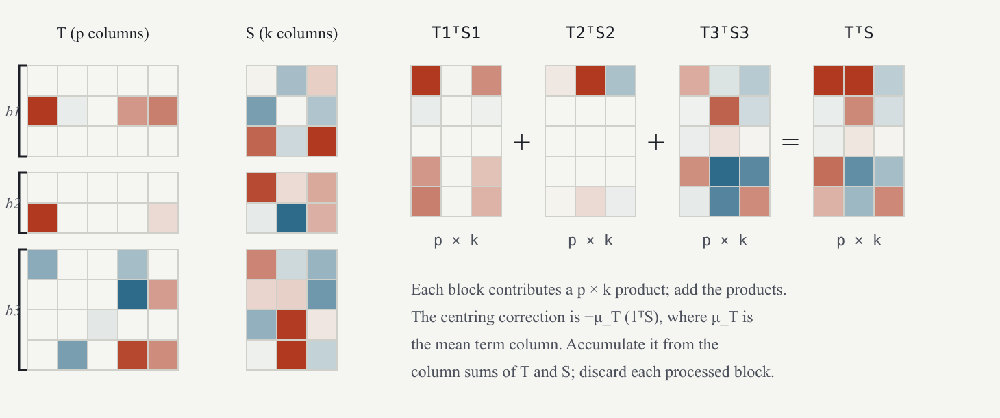
Let $N_b$ count articles in block $b$, and let $T_b$ and $S_b$ contain its matching rows, with shapes $N_b\times p$ and $N_b\times k$. Write $\mathbf1_b$ for the $N_b\times1$ column of ones, while $\mathbf1$ without a subscript has length $N$. Then

$$T^{\top}S=\sum_b T_b^{\top}S_b,\qquad \mathbf1^{\top}S=\sum_b\mathbf1_b^{\top}S_b,$$ $$\mu_T=N^{-1}\sum_b T_b^{\top}\mathbf1_b.$$

Read these formulas as three accumulation tasks. First multiply matching term and score rows to update the cross-product. Second add term columns to update their sums. Third add score columns to update their sums. Also retain the total row count so the final term sums can be divided by $N$. The final mean and centering correction are computed after the block summaries have been combined, using the same unweighted naming convention as the full matrix.

Each block therefore contributes three small numerical arrays: a $p \times k$ matrix ($50{,}000 \times 60$, twenty-four megabytes), the column sums of its term rows ($p$ numbers) and the column sums of its scores ($k$ numbers). The block itself—the sparse rows of one month’s articles and their scores—is built, folded in, and dropped (Figure 18). The full $T$, which has 455 million non-zero entries for the 175-year corpus and was being held twice by the batch code, never exists in the naming pass. At the end the three accumulated pieces are combined by the formula above; a property test checks that the result equals the whole-matrix operator applied to the concatenated blocks, to $10^{-12}$.

The same pass over a block also projects its embeddings to coordinates and computes $T^2$, $Q$ and $\nu$ for its documents, writing them to the partition’s own table. The whole eigen fit is thus three passes over the archive—covariance, orientation, measurement—each of which reads one partition at a time. On 16.5 million articles it runs in ten minutes and stays at 0.3 GB of memory.

11.5 Stories one month at a time

Clustering into stories (chapter The clustering thresholds) is done within a day, and threading into episodes links a day’s stories to the previous day’s. For the clustering and episode-linking calculation, the dependency of day $\tau$ is on that day’s articles and the previous day’s story state. The carried state includes centroids and episode identities, which summarize the thread inherited from earlier days. It is not necessary to reload every earlier article. Other tasks, such as finding long-range precedents, have broader dependencies and are not covered by this particular memory reduction. The batch code loaded every article’s vector and title before starting; the streaming version walks the months in order, loads one month’s articles, clusters its days in sequence, carries the last day’s stories across the month boundary, writes the month’s stories and drops the month. Memory is one month of articles instead of 175 years of them. The month boundary is only a storage boundary: preserve the previous day’s state when crossing it, or an ongoing episode would be split accidentally. The notebook processes the same six synthetic days once as a full batch and once as two blocks, checking that the resulting episode identities agree.

11.6 What still has to fit in memory

A matrix’s shape tells us how many numerical entries it contains. A dense $p\times k$ accumulator has $pk$ entries. With eight-byte floating-point values, the $50{,}000\times60$ loading accumulator needs $50{,}000\times60\times8=24{,}000{,}000$ bytes, or 24 decimal megabytes. Each simultaneous worker needs its own accumulator unless the implementation arranges shared updates. A decimal megabyte is one million bytes; a gibibyte uses $2^{30}$ bytes, so unit labels matter when comparing reported memory.

This size calculation concerns numerical entries only. Sparse indices, object metadata, temporary arrays, and stored text consume additional memory. A measured process total cannot generally be obtained by multiplying a single matrix shape.

Two stages remain large. Randomized LSA uses a $p\times l$ working matrix $\Omega$, where $l$ is the chosen working width, normally larger than the final retained rank. Products such as $T\Omega$ and $T^{\top}(T\Omega)$ are the range-finding operations described in §5, with the required centering and weighting corrections. The first product can be emitted by row block; the second is a sum of block cross-products. This avoids requiring all of $T$ at once, although working score matrices also need a storage plan. In the reported edition the 455-million-nonzero matrix remains in memory: 31 GB on a 64 GB laptop. The block form is a next step, not a claimed implementation. The other large object is the site index, which retains story centroids and profiles for precedents: about 20 GB for 13.4 million stories. These retained objects determine the second edition’s build-machine requirement.