4 The covariance and its eigenvectors

4.1 Centering and covariance

4.1.1 From an average to a measure of spread

The mean is an average: add the observations and divide by their count. For the scalar values 1, 2, and 3, the mean is $(1+2+3)/3=2$. Their deviations are the observed values minus that mean: −1, 0, and 1. Subtracting a common reference mean is called centering. The centered values say where each observation lies relative to that reference rather than relative to zero on the original scale.

Adding signed deviations gives zero here. That does not mean there is no spread; the negative and positive deviations cancel. Squaring avoids this cancellation. The squared deviations are 1, 0, and 1, whose mean is $2/3$. This average squared deviation is the variance under the total-count convention used for the fitted covariance. Its nonnegative square root, $\sqrt{2/3}\approx0.8165$, is the standard deviation. If observations are measured in some unit, variance is measured in that unit squared; standard deviation returns to the original unit.

Some statistical estimates divide the sum of squared deviations by one less than the count, to correct a bias when estimating a population variance from a sample. That is a different convention. The fitted covariance below divides by total weight. We will identify the reference and divisor when using a standard deviation elsewhere.

4.1.2 How two coordinates vary together

For more than one coordinate, calculate a mean for each coordinate. Consider the two observation rows $(1,2)$ and $(3,4)$. Their mean row is $(2,3)$, and their centered rows are $(-1,-1)$ and $(1,1)$. The first-coordinate squared deviations average to 1; the second-coordinate squared deviations also average to 1. The products between the first and second deviations are $(-1)(-1)=1$ and $(1)(1)=1$, so their average is also 1.

That last average is the covariance between the two coordinates. It is positive when deviations tend to have matching signs, negative when they tend to have opposite signs, and zero when their average product is zero. Statistical independence means that knowing one variable supplies no information about the other. Zero covariance does not generally establish independence: two variables may still have a relationship that this signed product does not detect.

Arrange these averages in a table. Diagonal entries compare a coordinate with itself and are variances; off-diagonal entries are covariances. For the two-row example the table is

$$\begin{pmatrix}1&1\\1&1\end{pmatrix}.$$

To compute every pairwise product at once, place a centered observation in a column and multiply it by its transpose. This outer product produces a square table. Its entry in row $j$, column $l$ is the product of centered coordinates $j$ and $l$. The two indices select coordinates, not articles. Averaging these tables produces the covariance matrix.

4.1.3 Fit weights change the average, not the operation

Let $i$ index fitted articles, from 1 to $n$, and let $d$ count embedding coordinates. Each $x_i$ is a $d\times1$ column; row $i$ of the $n\times d$ data matrix $X$ is $x_i^{\top}$. Let $w_i$ be its nonnegative fit weight. A weighted mean gives each observation the stated weight, adds the weighted contributions, then divides by the total weight. Let $Z>0$ be that total and $\mu$ the $d\times1$ weighted mean. A sum over $i$ includes every fitted article, and $Z^{-1}$ means $1/Z$:

$$Z = \sum_i w_i, \qquad \mu = Z^{-1} \sum_i w_i x_i,$$

For example, give the two observation rows above weights 1 and 3. The total is 4, the first mean coordinate becomes $(1\times1+3\times3)/4=2.5$, and the second becomes 3.5. Centering must use this new weighted mean. The centered rows are $(-1.5,-1.5)$ and $(0.5,0.5)$. The weighted mean of either squared coordinate is $(1\times2.25+3\times0.25)/4=0.75$. Every entry of this example’s weighted covariance is 0.75.

Let $\Sigma$ name the $d\times d$ weighted covariance. Apply precisely the same weights to the outer products of deviations from the weighted mean:

$$\Sigma = Z^{-1} \sum_i w_i (x_i - \mu)(x_i - \mu)^{\top}.$$

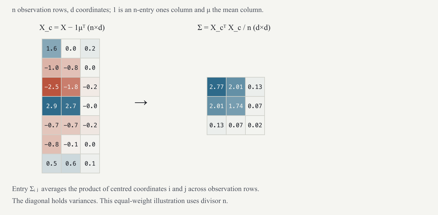
The first edition uses uniform article weights; the later archive fit uses inverse daily article counts, explained in §11. These weights are distinct from the story energy used to rank news. In Eigen Times $d=384$, so $\Sigma$ is a $384\times384$ matrix—147,456 numbers summarising the fitted article cloud. Figure 4 pictures the operations in their working order: center each observation, take its outer product, and average the products.

4.1.4 Why three sums suffice to update the covariance

A practical point matters for updates. Let $m$ be the $d\times1$ weighted coordinate sum and $M$ the $d\times d$ weighted outer-product sum:

$$m=\sum_i w_i x_i,\qquad M=\sum_i w_i x_i x_i^{\top}.$$

The mean is immediately $m/Z$. To recover covariance, first expand a single centered outer product:

$$(x_i-\mu)(x_i-\mu)^{\top} =x_ix_i^{\top}-x_i\mu^{\top}-\mu x_i^{\top}+\mu\mu^{\top}.$$

Now take the weighted average of all four terms. The first becomes $M/Z$. In the second and third terms, the weighted average of $x_i$ is $\mu$, so each becomes $-\mu\mu^{\top}$. The last term is the same for every observation and averages to $+\mu\mu^{\top}$. Two subtractions and one addition leave one subtraction:

$$\mu=m/Z,\qquad \Sigma=M/Z-\mu\mu^{\top}.$$

The three running sums $Z,m,M$ therefore retain everything needed for these mean and covariance calculations. They do not retain the full article collection. New observations with fixed weights can be added without revisiting old observations. If a day’s final article count changes its existing weights, the old contributions must also be corrected. Although the identity is exact, subtracting large nearly equal floating-point numbers can lose accuracy; the streaming chapter distinguishes algebraic identities from numerical reliability.

For compact matrix notation, let $W=\mathrm{diag}(w_1,\ldots,w_n)$ be the $n\times n$ diagonal weight matrix: $\mathrm{diag}$ puts the listed values on the diagonal and zeros elsewhere. Let $\mathbf1$ be a column of $n$ ones. Multiplying $\mathbf1\mu^{\top}$ repeats the mean row $n$ times. The centered data matrix is therefore $X_c=X-\mathbf1\mu^{\top}$. Multiplying $WX_c$ scales each centered row by its weight; multiplying on the left by $X_c^{\top}$ then sums the weighted products. This gives the same covariance as $\Sigma=X_c^{\top}WX_c/Z$.

4.2 Eigenvectors: the axes of the cloud

A cloud of points in $d$ dimensions has a shape. It can be broad in one direction and narrow in another, even when neither direction follows an original coordinate axis. We want to measure that shape using perpendicular directions. The special directions of the covariance matrix will supply them.

A nonzero $d\times1$ column $v$ is an eigenvector of $\Sigma$ with eigenvalue $\lambda$ when $\Sigma v=\lambda v$. The left side multiplies the vector by a matrix; the right side multiplies it by a scalar. Equality says that this input stays on its own line under the matrix operation. For a positive eigenvalue it points the same way and changes length by that factor; a zero eigenvalue sends it to zero.

4.2.1 Check an eigenpair by multiplication

Consider the separate exact example

$$\Sigma=\begin{pmatrix}2&1\\1&2\end{pmatrix}.$$

Multiplying by $(1,1)^{\top}$ gives $(3,3)^{\top}=3(1,1)^{\top}$. Multiplying by $(1,-1)^{\top}$ gives $(1,-1)^{\top}=1(1,-1)^{\top}$. We have found two eigendirections and eigenvalues 3 and 1. Their dot product is zero. Their lengths are both $\sqrt2$, so divide each by $\sqrt2$ to obtain unit columns, called $v_1$ and $v_2$. Scaling an eigenvector to unit length does not change its eigenvalue.

This is a way to verify an answer, not an assumption that every covariance’s eigenvectors are easy to guess. Numerical algorithms find them for larger matrices. The purpose of the example is to make the equation an operation we can inspect.

For a covariance, eigenvalues are nonnegative. Here is why. Let $u$ be any unit column direction and let $a_i=u^{\top}(x_i-\mu)$ be observation $i$’s scalar projection score along it. Its weighted mean is zero because the observations were centered. Its weighted variance is the average squared score. Substituting the covariance definition gives

$$Z^{-1}\sum_i w_i a_i^2=u^{\top}\Sigma u.$$

The left side is an average of nonnegative squares. If $u$ is a unit eigenvector with eigenvalue $\lambda$, the right side becomes $u^{\top}(\lambda u)=\lambda(u^{\top}u)=\lambda$. Thus the eigenvalue is exactly the variance along that unit direction and cannot be negative.

4.2.2 Write the whole covariance in its own directions

Choose $d$ unit, mutually perpendicular eigenvectors $v_j$, ordered by decreasing eigenvalue $\lambda_j$, with $j=1,\ldots,d$. Real symmetric matrices permit such a choice, although repeated eigenvalues need not specify unique individual directions. Let $V$ contain those columns and $\Lambda$ the diagonal matrix of their eigenvalues, both $d\times d$. They diagonalise the covariance, meaning

$$\Sigma = V\Lambda V^{\top},\qquad V^{\top}V=I,\qquad \Lambda=\mathrm{diag}(\lambda_1,\ldots,\lambda_d),$$

where $\lambda_1\ge\lambda_2\ge\cdots\ge\lambda_d\ge0$ and $\ge$ means greater than or equal to. The diagonal representation has zero covariances between different eigenvector coordinates. The principal components are these directions, ranked by variance; using them to summarize the cloud is principal component analysis (PCA).

Read the factorization from right to left when applying it to a column: $V^{\top}$ expresses the input in eigenvector coordinates, $\Lambda$ scales each coordinate separately, and $V$ expresses the result back in the original coordinates. The covariance is simple in this basis because no off-diagonal terms mix the coordinates.

Why does the first direction capture the most variance? Express an arbitrary unit direction as a combination $u=\sum_j\alpha_jv_j$, where each scalar $\alpha_j$ is its coordinate in the full orthonormal eigenbasis. Its unit length means $\sum_j\alpha_j^2=1$. Its projected variance becomes

$$u^{\top}\Sigma u=\sum_j\lambda_j\alpha_j^2.$$

The squared coordinates are nonnegative and add to one. The variance is therefore a weighted average of the eigenvalues and cannot exceed the largest, $\lambda_1$. Choosing $u=v_1$ reaches that largest value. Requiring the next direction to be perpendicular to $v_1$ sets its first coordinate to zero; the same argument then selects $v_2$. This explains the ordering without assuming calculus.

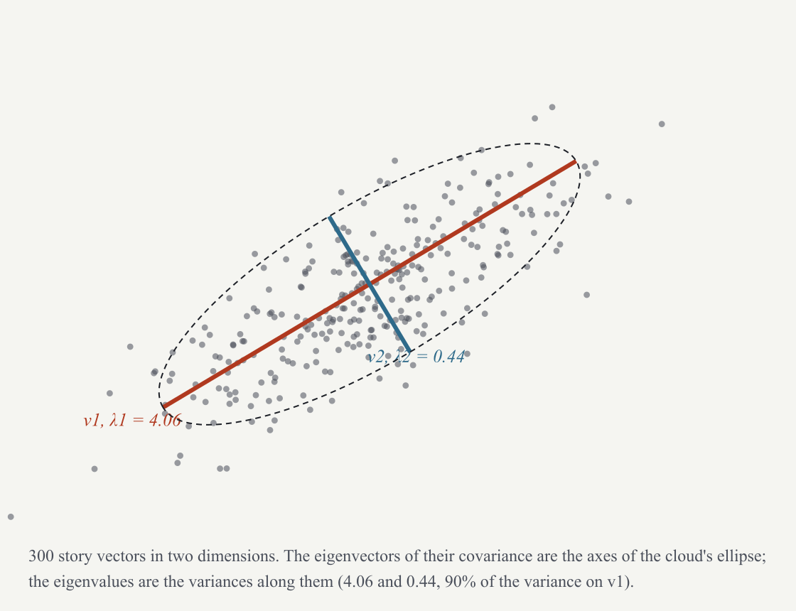
Figure 5 shows 300 points in two dimensions: the long axis has eigenvalue 4.06, the short one 0.44, so about 90% of the displayed variation lies along one direction. The synthetic distribution has known mean zero. This illustration forms second moments about that origin, rather than subtracting the finite sample’s empirical mean; the displayed eigenvalues estimate population variances. The notebook computes both choices so that centering is an explicit decision.

This is the content of “the eigen‑news are the directions that explain the most variance”. Variance describes spread in the chosen numerical representation; the argument alone does not establish significance, truth, or editorial importance. Computing eigenvectors for a $384\times384$ symmetric matrix is a standard numerical operation (eigh in common linear-algebra libraries; faer in the Rust implementation) and takes milliseconds in the reported fit.

4.3 How many axes to keep

Let $k\le d$ count retained directions; $\le$ means less than or equal to. The explained-variance fraction is $\sum_{j=1}^{k}\lambda_j/\sum_{j=1}^{d}\lambda_j$, provided total variance is positive. It reports how much of the fitted cloud’s variation those directions retain. For the Eigen Times embedding basis, 60 components carry 55% of the variance, and the curve is flat beyond; a small eigenvalue alone does not prove that a direction is meaningless.

In the exact two-direction example, total variance is $3+1=4$. Keeping the first direction retains $3/4=75\%$ and discards $1/4=25\%$. Keeping both retains all the variance. With a longer list of eigenvalues, make the same running calculation: add the retained values, divide by the sum of all values, and inspect what each extra direction contributes. A flat part of that curve means that each new direction adds little to the numerator. It does not mean that the discarded articles or subjects are unimportant.

The Marchenko–Pastur edge asks a different question: how large might covariance eigenvalues be in a specified model of featureless variation? Here noise means variation generated by that reference model, not a judgment about an article. The spectrum of a covariance is its collection of eigenvalues. In this illustration, let $N$ count independent observations in $d$ coordinates with equal noise variance $\sigma^2$, unrelated to the singular-value notation used later. For a concrete reference, suppose all entries are independent draws from the same zero-mean Gaussian distribution, a symmetric bell-shaped probability model, with variance $\sigma^2$. Independence applies across both observations and coordinates; repeated draws use the same distribution. These assumptions specify an illustrative noise model, not a description of news embeddings. Let $\lambda_+$ denote the approximate upper edge of the model’s covariance spectrum. Under that model, in the large-sample limit,

$$\lambda_{+} = \sigma^2 \left(1 + (d/N)^{1/2}\right)^2,$$

Here raising to $1/2$ means taking a square root. First form the dimension-to-observation ratio $d/N$, take its square root, add one, square, and multiply by the stipulated variance. The notebook uses $\sigma^2=0.01$, $N=1{,}000{,}000$, and $d=384$, giving approximately 0.010396. That is slightly larger than 0.01: finite sampling can spread estimated variances even when the model gives every coordinate the same underlying variance. This teaching input is not an estimate fitted to news.

Eigenvalues near or below such a reference may be noise; this is not a universal significance test for correlated, weighted news data. The median eigenvalue supplies a rough noise-variance estimate in the reported comparison. With $N\approx10^6$ and $d=384$, the ratio $d/N$ is tiny and the edge is close to that estimate. The deployed bases use fixed $k=60$, with the variance curve as a check. From here onward $V$ usually means only the retained $d\times k$ columns and $\Lambda$ their $k\times k$ positive eigenvalue matrix; full decompositions will be identified explicitly.