6 From eigenvectors to named axes

6.1 Two ambiguities

Eigenvectors come with two kinds of freedom that the mathematics does not fix and a newspaper must.

6.1.1 Choose which end of an axis points positive

If $v$ is an eigenvector, so is $-v$: the same line pointing the other way. A score is measured by a dot product with the direction, so flipping the direction also flips its scores. The contribution to reconstruction is unchanged because $(-v)(-c)=vc$ for a scalar score $c$. Its positive and negative poles, the two ends of the line, exchange names. Choosing a sign gives the display a consistent convention without changing the represented observations.

Eigen Times fixes orientation using skewness, a measure of asymmetry in the score distribution. Here a distribution describes how frequently different score values occur, and a tail is the part extending toward unusually large or small scores. A central moment averages powers of deviations from the mean. We already know the second central moment: averaging squared deviations gives variance. The third central moment instead averages cubed deviations. Cubing retains signs, so a large negative deviation contributes negatively and a large positive deviation contributes positively.

Let $m_2$ and $m_3$ denote the second and third central moments on one axis. For the notebook’s scores −5, −1, 0, 1, 1, the mean is −0.8. The centered scores are −4.2, −0.2, 0.8, 1.8, 1.8. Squaring and averaging gives $m_2=4.96$; cubing and averaging gives $m_3=-12.384$. The negative third moment says that, by this signed cubic measure, the negative side is more pronounced.

When $m_2>0$, standardized skewness is $m_3/m_2^{3/2}$. The power $3/2$ means the standard deviation cubed: $m_2^{3/2}=(\sqrt{m_2})^3$. This division removes the units of the scores, but it does not change the sign. The orientation rule therefore needs only the sign of $m_3$: flip if $m_3<0$, making the third moment positive. Reversing all centered scores preserves their squares and reverses their cubes. This is a convention based on the measured third moment, not a claim that every asymmetric distribution has one unambiguous longer tail. A zero third moment supplies no preferred sign. The streaming chapter computes these moments without retaining every score.

6.1.2 Choose directions inside an already selected subspace

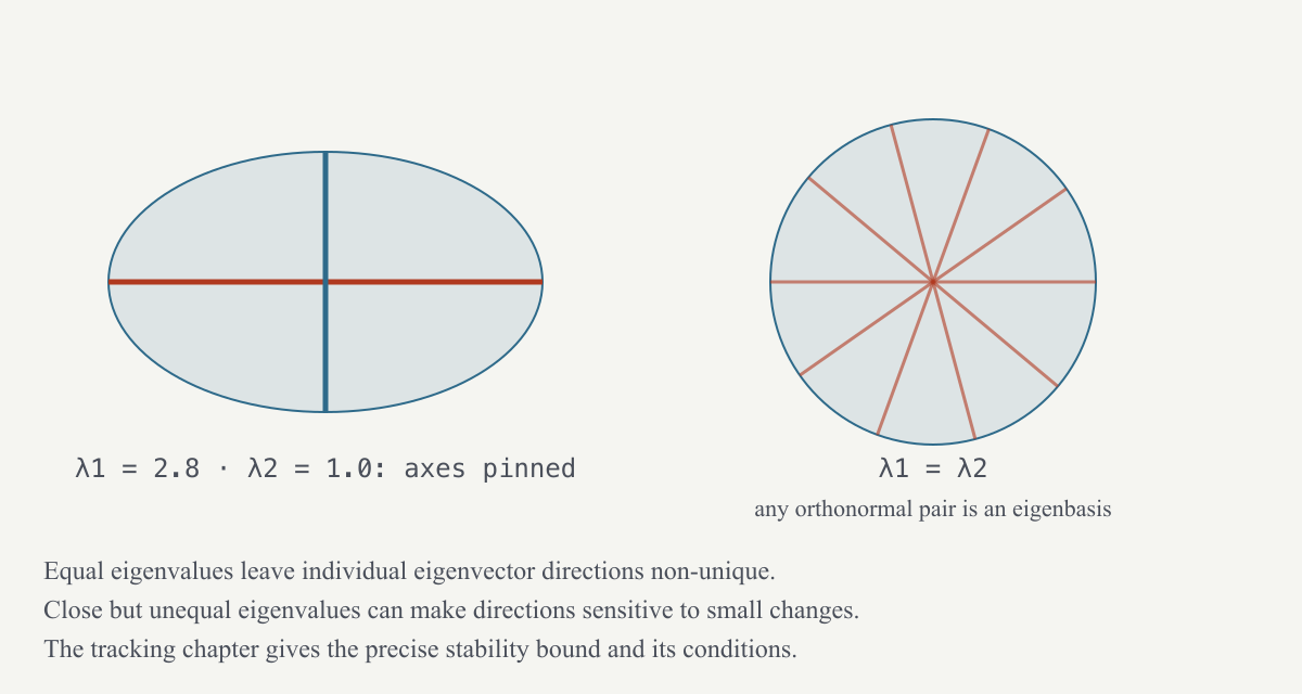
Equal eigenvalues are called degenerate: any perpendicular unit pair in their plane is an eigenbasis. For example, a covariance equal to twice the identity multiplies every direction by two. There is no uniquely preferred diagonal in its plane because every unit direction has variance two. The notebook rotates this covariance and verifies that its entries remain unchanged.

Close eigenvalues can make individual directions sensitive to small data changes, even when their shared subspace is stable (Figure 9). A perturbation is such a change to the covariance; the eigenvalue gap is the separation from neighbouring eigenvalues. The tracking chapter explains the bound relating them. Even distinct principal axes can be difficult to name: variance-maximising directions may blend subjects such as markets and party politics. Naming keeps the selected subspace and chooses different axes inside it; the rotated axes need no longer be covariance eigenvectors. The purpose of the new coordinates is readability, while the retained geometric information stays the same.

6.2 Varimax

6.2.1 Turn the axes and counter-turn the coordinates

Recall the retained $d\times k$ orthonormal basis $V$. Let $R$ be a $k\times k$ orthogonal rotation and let $V'=VR$ be the named basis; the prime here means rotated. If $c$ is a $k\times1$ raw coordinate column, its named column is $y=R^{\top}c$ (also sometimes written $c'$). Why does the coordinate transformation use the transpose? The coordinates must change oppositely to the basis so that the represented point stays fixed. Substituting $y$ and using $RR^{\top}=I$ gives

$$V'y=VR(R^{\top}c)=Vc.$$

Both bases therefore reconstruct the same projection. Subtracting that same projection from an observation leaves the same residual, so its length is unchanged. The covariance-adjusted distance called $T^2$ in §7 is also unchanged when its covariance is transformed consistently; it is not determined by the subspace alone.

6.2.2 Read the criterion as a variance calculation

Kaiser’s varimax criterion selects a rotation making each direction load strongly on some features and weakly on others. A criterion, or objective, is a numerical rule for comparing candidate choices. A larger value of this criterion indicates greater contrast in the sizes of loadings within the columns. It favors concentration but does not force entries to become exactly zero.

Let $p$ count the features, let $i=1,\ldots,p$ index them, and let $j=1,\ldots,k$ index axes. Write $\ell_{ij}$ for row $i$, column $j$ of the rotated loading table. Hold one column $j$ fixed. Square each loading, average those squared loadings, then measure how much the squared loadings vary around their mean. Squaring treats equally strong positive and negative loadings equally; it is concentration of magnitude that matters here.

We already derived the identity “variance equals mean square minus square of mean.” Apply it to the values $\ell_{ij}^2$. Their squares are $\ell_{ij}^4$, so this column’s variance is the average fourth power minus the square of the average second power. Add those variances over columns. That sequence of operations gives the criterion

$$\sum_{j=1}^{k}\left[\frac1p\sum_{i=1}^{p}\ell_{ij}^{4}-\left(\frac1p\sum_{i=1}^{p}\ell_{ij}^{2}\right)^2\right].$$

The fourth power appears because it is the square of a squared loading. It is not a new assumption that extreme feature values should be counted four times. For a two-feature column with loadings 1 and 0, squared loadings are 1 and 0, their mean is 0.5, and the variance of those squared loadings is $((1-0.5)^2+(0-0.5)^2)/2=0.25$. Spread the same total squared loading equally by using loadings $1/\sqrt2$ and $1/\sqrt2$. The squared loadings are now 0.5 and 0.5, so their variance is zero. The first column has greater concentration even though both columns have squared length one. In a rotation we cannot choose each column independently: the whole loading table must turn together. The notebooks compute the variance of squared loadings by directly subtracting each column’s mean and also by the displayed formula; the two methods agree.

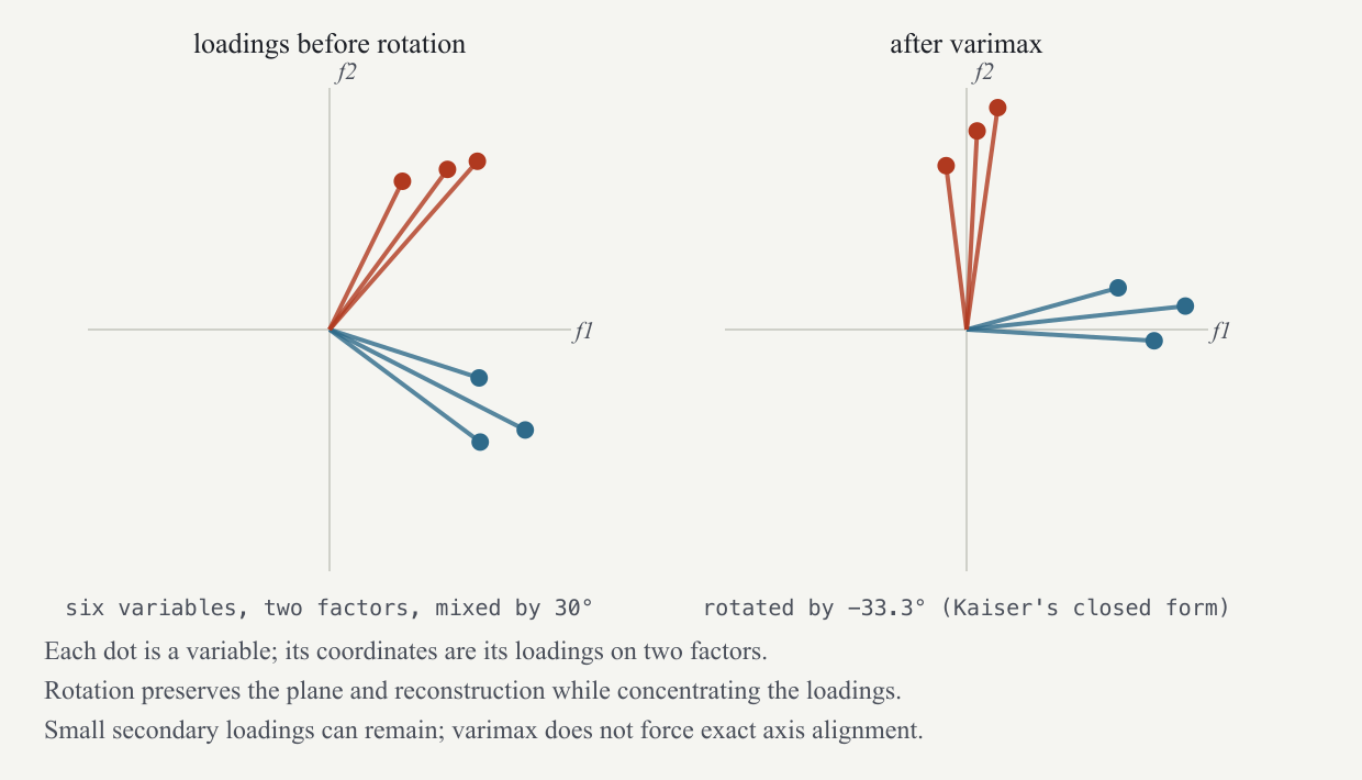
Figure 10 shows six variables in two groups mixed by 30°. Their small secondary loadings make the computed maximizing rotation approximately $-33.3°$, rather than an exact reversal of the mixing angle. The rotation concentrates each variable on one axis without making its other loading exactly zero.

6.2.3 Rotate two columns at a time

Eigen Times sweeps over every pair of axes, rotating just that pair by its best angle. This two-coordinate operation is a Givens rotation. It leaves the other columns unchanged, reducing one step of a many-axis search to choosing one angle.

Let $\phi$ (Greek phi) denote that angle. Angles may be measured in degrees, with 360° in a full turn, or in radians, where angle is arc length divided by circle radius. One full turn is $2\pi$ radians, with $\pi$ the circle constant. On the unit circle, $\cos\phi$ is the horizontal coordinate and $\sin\phi$ the vertical coordinate after turning through $\phi$ from the positive horizontal direction. Their squared sum is 1 because the point lies on that circle. A two-dimensional rotation matrix is

$$R(\phi)=\begin{pmatrix}\cos\phi&-\sin\phi\\\sin\phi&\cos\phi\end{pmatrix}.$$

For one pair only, let $x,y$ be its $p\times1$ loading columns, distinct from article and score vectors elsewhere. Multiplying the loading table by $R(\phi)$ changes row $i$’s pair to

$$x_i\cos\phi+y_i\sin\phi,\qquad -x_i\sin\phi+y_i\cos\phi.$$

These two entries’ squared sum remains $x_i^2+y_i^2$. Rotation redistributes a row’s contribution between axes while preserving its total squared size.

6.2.4 Why the best angle contains a quarter of an angle

We can evaluate the criterion for many trial angles, but the two-column case also has a direct formula. Elementwise arithmetic treats each row separately. Define $u_i=x_i^2-y_i^2$ as the difference of the squared loadings and $v_i=2x_iy_i$ as twice their product. Define four scalar sums

$$A=\sum_i u_i,\quad B=\sum_i v_i,\quad C=\sum_i(u_i^2-v_i^2),\quad D=\sum_i2u_iv_i.$$

These local capital letters are scalars, not earlier matrices. The first two sums measure the column totals of the new quantities; the last two collect their squared and cross-product terms. Define centered combinations $C_*=C-(A^2-B^2)/p$ and $D_*=D-2AB/p$. The subscript star marks these adjusted scalar values.

Here is the route from the criterion to the angle. After rotation, the difference of the two squared loadings is $u_i\cos(2\phi)+v_i\sin(2\phi)$, obtained by expanding the two squared rotated entries and using the double-angle identities. In those identities, $\cos(2\phi)=\cos^2\phi-\sin^2\phi$ and $\sin(2\phi)=2\sin\phi\cos\phi$. Substituting this difference into the variance criterion and expanding once more leaves an angle-independent part plus

$$\frac{C_*\cos(4\phi)+D_*\sin(4\phi)}{4p}.$$

The appearance of $4\phi$ comes from squaring expressions that already involve $2\phi$. We can maximize the displayed part geometrically: it is a dot product between the fixed vector $(C_*,D_*)$ and the unit vector $(\cos(4\phi),\sin(4\phi))$, divided by a positive constant. The dot product is largest when the unit vector points along the fixed vector. The function $\operatorname{atan2}(a,b)$ returns the angle of the point with horizontal coordinate $b$ and vertical coordinate $a$, preserving the quadrant that a ratio alone would lose. It supplies $4\phi$; divide by four to get

$$\phi = \tfrac{1}{4}\,\operatorname{atan2}\left(D - 2AB/p,\; C - (A^2 - B^2)/p\right).$$

This is a formula for choosing a maximizing angle, not a requirement to memorize trigonometric manipulation. The notebooks check its objective against a dense grid of trial angles and verify the angle-dependent expression. If both arguments of $\operatorname{atan2}$ are zero, that expression is constant and the pair supplies no preferred rotation.

A sweep visits every axis pair. Sweeps stop when no pair rotates by more than $10^{-6}$ radians (one millionth of a radian), or after fifty sweeps. Exact pairwise maximization cannot decrease the criterion, so its bounded objective improves monotonically, meaning it never moves downward. This does not guarantee the global best orientation: the choices across many column pairs interact. The reported alternative, an SVD-based fixed-point iteration (repeatedly applying one update rule), oscillated between two mirror-image states on a symmetric configuration, motivating the pairwise method.

6.2.5 Give an embedding direction evidence from words

For the embedding basis, naming rotates associations with words rather than unexplained embedding coordinates. The articles supply the common rows connecting the two descriptions: each has term measurements and raw eigen-coordinates.

Let $T$ be the $N\times p$ article TF‑IDF matrix, $\mu_T$ its $p\times1$ article mean, and $\mathbf1$ a column of $N$ ones. Let $S$ be an $N\times k$ table of raw eigen-coordinates divided by their positive raw-axis standard deviations. Dividing a coordinate by its standard deviation makes one unit mean one reference standard deviation on every axis. Because the unrotated eigen-coordinates already have zero reference mean and zero reference cross-covariance, this scaling gives unit reference variance and zero reference cross-covariance. Together those properties are called whitening. Scaling arbitrary correlated coordinates to unit variance would not by itself remove their cross-covariances.

Let $\beta$ (Greek beta) be the $p\times k$ term-loading matrix. Its entry for one term and one axis sums, over articles, the centered term value multiplied by that article’s standardized raw score. Positive products arise when the term and score are both above their respective references, or both below. The sum measures association between term use and the direction; it is not a probability and has not been divided by the number of articles. Matrix multiplication performs all these sums together:

$$\beta=\left(T-\mathbf1\mu_T^{\top}\right)^{\top}S.$$

Here $p=50{,}000$ and $k=60$. Lexical whitening floors its raw variance denominators at $10^{-12}$ before taking square roots: if a variance is smaller, the implementation uses that positive minimum to avoid division by zero or an excessively small scale. Exact unit-variance whitening applies to positive axes whose denominators have not been changed by this safeguard, under the same reference weights used to fit them.

The embedding naming fit rotates $\beta$; the LSA fit rotates its right singular directions, already indexed by terms. Applying the resulting $R$ to the corresponding raw coordinate map gives named directions. Because scaling and rotation need not give the same result in opposite orders, word associations fitted from whitened scores are labels for investigation, not exact term-by-term decompositions of every stored named score. The block-sum chapter expands the centered loading formula. The older shorthand $T^{\top}U$ assumes compatible centered, scaled score columns; the SVD factor $U$ must not generally be substituted for $S$. The distinction is practical: a unit left singular direction, an article coordinate, and a variance-standardized coordinate carry different scales even when they point along related patterns.