5 A population of profiles makes a people basis

5.1 Center the rows around the population

Let $n$ now count the fitted people, so $B$ has shape $n\times K$. Its rows have unit length, but they need not average to zero. Denote their $1\times K$ mean row by $\bar b$. In the example it is

$$\bar b\approx(0.1276,0.0652,0.1407).$$

Let $\mathbf1$ denote a column of $n$ ones, so $\mathbf1\bar b$ repeats the mean row for every person. Subtract it from $B$ and call the resulting $n\times K$ centered matrix $H$:

$$H=B-\mathbf1\bar b.$$

Let $h_p=b_p-\bar b$ denote person $p$’s row of $H$. For A,

$$h_A=b_A-\bar b\approx(0.3411,-0.6500,0.5213).$$

This second centering asks how A’s normalized coverage differs from the fitted population of normalized person profiles. The earlier subtraction compared articles inside a cell. The reference objects are different.

5.2 Covariance asks which coordinates move together

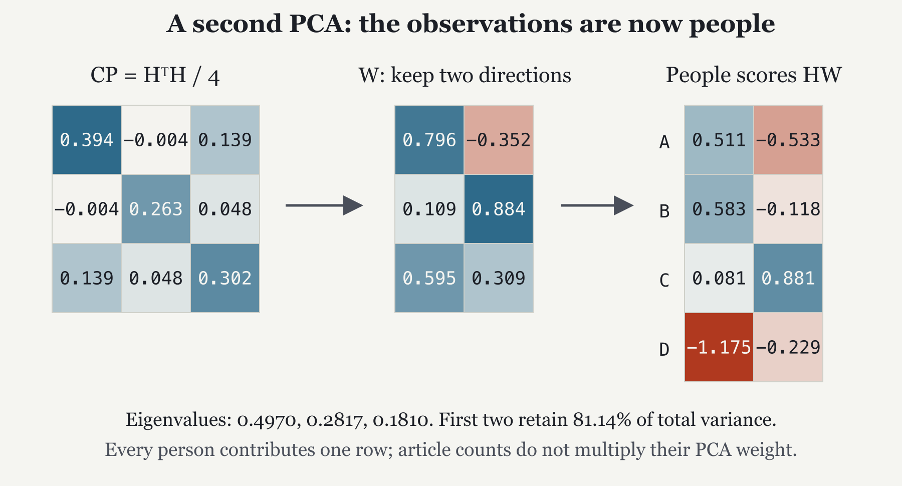
Let $C_P$ denote the $K\times K$ people covariance. Using the fitted-person count $n$, compute it as

$$C_P=\frac1nH^{\mathsf T}H,$$

Here $j$ and $k$ each index news coordinates from 1 to $K$. Entry $(j,k)$ is the average product of those two centered coordinates across people. A large positive product tends to occur when both coordinates deviate in the same direction; a negative product occurs when they deviate oppositely. The diagonal entries are coordinate variances.

Each person contributes one row. A person supported by 10,000 articles does not enter the covariance a thousand times more heavily than a person supported by ten. More articles can affect the quality of a row, but they are not its weight in this fit. This is equal-person PCA: principal component analysis of normalized, centered coverage profiles.

Let $\ell$ index a people direction, $w_\ell$ its $K\times1$ unit eigenvector column, and $e_\ell$ its covariance eigenvalue. Each pair satisfies

$$C_Pw_\ell=e_\ell w_\ell.$$

Multiplying the direction by the covariance stretches it by $e_\ell$ without turning it. As explained in the Eigen Times eigenvector chapter, the largest eigenvalue identifies the direction of greatest variation, and the next identifies the greatest variation perpendicular to it.

5.2.1 Read one matrix entry as an average

For the original four-person fixture, the first centered coordinate is approximately 0.3411 for A, 0.8207 for B, -0.3459 for C, and -0.8159 for D. The N1 variance therefore adds their four squares and divides by four, giving approximately 0.393847. The N1–N3 covariance instead multiplies each person’s first and third centered entries and averages the four products, giving approximately 0.138797. Both calculations use one product per person. The notebook prints the complete centered table and checks the covariance against independent reference entries.

5.2.2 Verify an eigenvector with two coordinates

Set the four-person matrix aside for a small covariance illustration. Let $C_*=\begin{pmatrix}2&1\\1&2\end{pmatrix}$. The star marks this separate synthetic table. Let $a_+=(1,1)^{\mathsf T}/\sqrt2$ and $a_-=(1,-1)^{\mathsf T}/\sqrt2$ be unit columns. Multiplying the first gives $(3,3)^{\mathsf T}/\sqrt2=3a_+$. Multiplying the second gives $(1,-1)^{\mathsf T}/\sqrt2=a_-$. They are eigenvectors with eigenvalues 3 and 1; their dot product is $(1-1)/2=0$.

For a unit column $a$, the scalar $a^{\mathsf T}C_*a$ is variance along that direction. Along the first coordinate axis it is 2. Along $a_+$ it is 3; along $a_-$ it is 1. To see why 3 is the maximum, express any unit direction as $a=\gamma a_++\delta a_-$, where $\gamma,\delta$ are scalar coefficients satisfying $\gamma^2+\delta^2=1$. Its variance is $3\gamma^2+\delta^2=1+2\gamma^2$, no larger than 3. The larger-eigenvalue direction captures the most spread because of this numerical property, not because its words are necessarily more important.

Multiplying an eigenvector by -1 leaves its line and eigenvalue unchanged. Its coordinates and resulting scores both reverse signs. A sign convention is useful for reproducible displays; it does not change the represented variation.

5.3 Keep two patterns in the toy world

The toy covariance has eigenvalues approximately $0.4970$, $0.2817$, and $0.1810$. Keeping the first two retains

$$\frac{0.4970+0.2817}{0.4970+0.2817+0.1810}\approx0.8114$$

of the between-person variance, or 81.14%. This is a reconstruction statement about this four-person cloud. It is not an accuracy estimate, an identity confidence, or the fraction of articles explained.

Let $r$ count the retained positive people directions; it is 2 in this toy example. The bare $r$ is a count, distinct from the contrast row $r_p$. The retained direction index $\ell$ runs from 1 to $r$. Put those eigenvectors, ordered by decreasing eigenvalue, into the columns of the $K\times r$ loading matrix $W$:

$$W\approx\begin{pmatrix} 0.7964&-0.3516\\ 0.1090&0.8838\\ 0.5949&0.3087 \end{pmatrix}.$$

Its rows correspond to N1, N2, N3; its columns correspond to people patterns P1 and P2. The columns have length one and are perpendicular. Their signs are oriented so the largest-magnitude news loading is positive, matching the implementation’s sign convention. Flipping a column and all its scores would describe the same geometry. When two eigenvalues are close, a small change in data can rotate their directions substantially even while their combined subspace changes little. Fixing signs does not remove that ambiguity; it is another reason to keep model versions explicit.

5.3.1 Account for the omitted variance

The three fitted eigenvalues sum to approximately 0.9596456. This is also the sum of the three diagonal entries of $C_P$, called its trace: total centered squared length per person, expressed in either coordinate system. The first two sum to approximately 0.7786802. Their ratio is 0.8114248; multiplying by 100 expresses it as a percentage. The omitted fraction is about 0.1885752.

The loading columns are unit directions, but a row of $W$ need not have length one. Similarly, the score rows need not be unit rows after population centering and projection. Keeping these distinctions prevents a loading, a coordinate, and a cosine from being treated as interchangeable numbers.

5.4 Locate a person on the patterns

Let $u_p$ denote person $p$’s $1\times r$ people-coordinate row. Project its centered profile $h_p$ onto the retained columns:

$$u_p=h_pW=(b_p-\bar b)W.$$

For A, the first coordinate is approximately

$$\begin{aligned} u_{A1}&\approx0.3411(0.7964)-0.6500(0.1090)\\ &\quad+0.5213(0.5949)\\ &\approx0.5109. \end{aligned}$$

The second uses the second column of $W$. The resulting rows are:

P1 is a pattern, not person D, although D has the largest absolute P1 score in this small example. A negative score identifies the other pole of a direction. It does not say that D is opposed to the other people.

In the published models, there are 60 news coordinates and at most 24 directions with positive eigenvalues. The 217-person Hacker News model retains 84.54% of between-person variance; the 61-person general-news model retains 90.86%. These separately fitted percentages should not be read as a contest between corpora. There is no second varimax naming step and no whitening of people scores. The people directions are orthonormal in standardized news coordinates, not generally when mapped back into the original embedding geometry.

5.4.1 Show both dot products

A’s first score adds approximately $0.2717-0.0709+0.3101=0.5109$. Its second coordinate is

$$\begin{aligned} u_{A2}&\approx0.3411(-0.3516)-0.6500(0.8838)\\ &\quad+0.5213(0.3087)\\ &\approx-0.1199-0.5745+0.1609\\ &\approx-0.5334. \end{aligned}$$

These are projections of the same centered row onto different direction columns. Small differences in final digits arise if we multiply displayed four-decimal entries rather than the full-precision fixture.

The first score column has variance 0.4970 and the second 0.2817, the eigenvalues already reported. They are not divided by the square roots of those variances in this model. Dividing them would whiten the retained scores and would change distances and cosines; that is a different geometry.