7 Returning through the map loses detail

7.1 The return operation

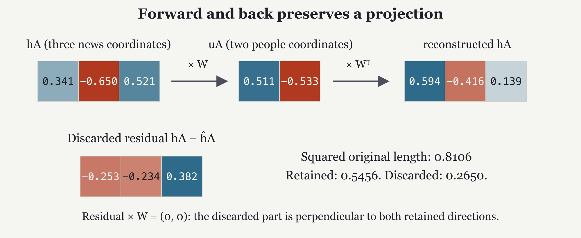
When discussing one person without naming them, write $b$, $h$, and $u$ for their unit profile $b_p$, centered profile $h_p$, and retained score row $u_p$. The rows $b,h$ have $K$ coordinates and $u$ has $r$. Let $\hat h$ be the $1\times K$ reconstruction of $h$; the hat denotes an approximation returned from retained coordinates. After calculating $u=hW$, multiply by the transpose:

$$\hat h=uW^{\mathsf T}=hWW^{\mathsf T}.$$

Adding $\bar b$ gives the corresponding reconstruction of the unit news profile. It does not give back the original articles.

An orthogonal projector keeps a vector’s component in a chosen subspace and discards its perpendicular component. Let $P$ be the $K\times K$ forward-and-return matrix, defined by $P=WW^{\mathsf T}$. A symmetric matrix equals its transpose; an idempotent matrix has the same effect when applied twice as once. Because the columns of $W$ are orthonormal, $P$ has both properties:

$$P^{\mathsf T}=P,\qquad P^2=W(W^{\mathsf T}W)W^{\mathsf T}=P.$$

The first equality expresses symmetry and the second idempotence. Together these identify an orthogonal projector. Once a row lies in the retained plane, projecting it onto that plane again changes nothing.

The residual is the difference between the original centered row and its reconstruction, $h-\hat h$. It is perpendicular to the retained directions. Consequently,

$$\lVert h\rVert^2=\lVert \hat h\rVert^2+\lVert h-\hat h\rVert^2.$$

This is the familiar right-triangle rule, now applied to components of a vector. In the fitted toy example, A’s discarded squared length is approximately 0.2650. The example script checks the decomposition and the orthogonality of the residual using unrounded values.

7.2 An even smaller exact example

To see the loss without decimals, set aside the fitted toy matrix for a moment. Let $W_*$ denote this deliberately chosen $3\times2$ matrix; the star distinguishes it from the fitted $W$:

$$W_* = \begin{pmatrix}1/\sqrt2&0\\1/\sqrt2&0\\0&1\end{pmatrix}.$$

This is an illustration, not another fit. It retains the shared direction of the first two coordinates and retains the third coordinate separately. A query $h=(1,0,0)$ goes forward to $(1/\sqrt2,0)$ and returns as $(1/2,1/2,0)$. The first-versus-second distinction was discarded.

A linear map preserves addition and scaling; multiplication by a fixed matrix is an example. An adjoint transfers a linear map to the other side of a dot product; for real matrices with Euclidean dot products, it is the transpose. Least squares means minimizing the sum of squared coordinate discrepancies. A Moore-Penrose pseudoinverse is a generalized inverse that gives least-squares solutions, choosing the shortest solution when several are possible. Because $W$ has orthonormal columns, $W^{\mathsf T}$ is both its adjoint and its pseudoinverse. It returns the least-squares reconstruction of a centered profile in the retained subspace. A two-sided inverse would undo the map in both directions for every input; this transpose cannot do that. With 24 retained directions out of 60, there is no way to recover every possible original 60-coordinate row.

7.2.1 Compute the residual and the shortest reconstruction

The first retained coordinate of $h=(1,0,0)$ is $1(1/\sqrt2)+0(1/\sqrt2)+0(0)=1/\sqrt2$; the second is zero. Returning multiplies the first column by $1/\sqrt2$, giving $(1/2,1/2,0)$. Subtraction leaves $(1/2,-1/2,0)$. Its squared length is $1/4+1/4=1/2$, and its dot products with both retained columns are zero. The returned part also has squared length $1/2$, so $1=1/2+1/2$.

Any alternative reconstruction inside the retained plane can be written $(t,t,s)$, where $t$ and $s$ are real scalar choices. Its squared discrepancy from $(1,0,0)$ is

$$\begin{aligned} (1-t)^2+t^2+s^2 &=2(t-1/2)^2+s^2+1/2. \end{aligned}$$

Squares cannot be negative, so the minimum is $1/2$, achieved at $t=1/2$ and $s=0$. This proves the least-squares claim for this example without asking the reader to trust an inverse formula.

7.3 Loss began before this projection

Even retaining every people direction would not recover an article list from a person profile. The earlier pipeline also reduced a 384-coordinate embedding to 60 news coordinates, averaged articles, subtracted backgrounds, and normalized lengths. Many different inputs can give the same output after those operations.

Navigation is valuable without being invertible. It provides linked views of a representation and routes back to stored evidence. The article links and factual sources are retained separately precisely because the vector cannot reconstruct them.

7.4 Why the singular value decomposition gives two views

Singular value decomposition (SVD) factors a matrix into two sets of orthonormal directions and nonnegative scale factors called singular values. For a longer prerequisite, revisit the Eigen Times SVD chapter. The operator $\min$ selects the smaller of two numbers. For the centered $n\times K$ matrix $H$, let $k_* = \min(n,K)$. In the thin decomposition, $U$ is an $n\times k_*$ matrix of left directions, indexed by people, and $Q$ is a $K\times k_*$ matrix of right directions, indexed by news coordinates. Both have orthonormal columns. Let $\Sigma$ be the $k_*\times k_*$ diagonal matrix of singular values in descending order. Then

$$H=U\Sigma Q^{\mathsf T}.$$

Recall that $r$ counts retained positive people directions. Let $U_r$ and $Q_r$ contain the first $r$ columns of their respective matrices, and let $\Sigma_r$ contain the leading $r\times r$ diagonal block of $\Sigma$. Thus $U_r$ has shape $n\times r$ and $Q_r$ shape $K\times r$. Using the same ordering and orientation as the people eigendecomposition gives $W=Q_r$ and

$$HW=U_r\Sigma_r.$$

The scores include the singular values; they are not just the columns of $U_r$. Each squared singular value divided by $n$ equals the corresponding eigenvalue of the earlier people covariance. The right directions come from $H^{\mathsf T}H$, while the left directions come from $HH^{\mathsf T}$. These are two sides of the same centered profile matrix. An adjacency matrix instead records which graph nodes have edges between them. Neither calculation uses that matrix from Anthropology’s relationship graph. A graph community is a group of nodes relatively densely linked to one another. Communities and people patterns can be interesting to compare, but they are not the same construction.

Check 6. For $W_*$ above, project $h=(0,1,0)$ forward and back. Compare its returned row with the return from $(1,0,0)$. What information can the map no longer distinguish?

7.4.1 A complete SVD that fits on a page

Use a separate centered table $H_*$ with four rows $(1,0)$, $(-1,0)$, $(0,2)$, and $(0,-2)$. Each column sums to zero. Multiplication gives $H_*^{\mathsf T}H_*=\operatorname{diag}(2,8)$: the first column’s squares sum to two, the second’s to eight, and their paired products are zero.

The largest right direction is therefore $(0,1)^{\mathsf T}$, followed by $(1,0)^{\mathsf T}$. The singular values are the square roots of eight and two: $\sqrt8$ and $\sqrt2$. Projecting the rows onto the first right direction gives $(0,0,2,-2)^{\mathsf T}$. Divide that column by $\sqrt8$ to obtain its unit left direction $(0,0,1/\sqrt2,-1/\sqrt2)^{\mathsf T}$. The second left direction is $(1/\sqrt2,-1/\sqrt2,0,0)^{\mathsf T}$.

Now multiply back: the first left column times $\sqrt8$ times the first right row restores only the second coordinate; the second term restores only the first coordinate. Adding the two restores every entry of $H_*$. With four observations, the covariance eigenvalues are $8/4=2$ and $2/4=0.5$. Keeping only the first singular direction retains $8/(8+2)=0.8$ of the total squared length. The discarded first-coordinate column has squared length two. This shows explicitly why scores contain singular values: the left direction has unit length, while its score column here has length $\sqrt8$.

The native OCaml teaching routine obtains a small SVD through a symmetric Gram matrix, the product $H_*^{\mathsf T}H_*$. That is adequate for these tiny well-scaled demonstrations; it is not presented as a numerically preferred algorithm for a large production fit. Both notebooks verify reconstruction, orthonormality, and the independent singular values.