3 Measuring an article on named news axes

3.1 First inherit a fixed news map

Eigen Times and Eigen Hacks turn an article’s text into an embedding, a list of numbers produced by a text model. Anthropology does not learn a new text embedding for every person. It inherits a versioned news coordinate system and measures each associated article in that system.

Let $a$ index an article and $d$ count embedding coordinates. Let $x_a$ be article $a$’s $1\times d$ embedding row, and $\mu$ the $1\times d$ mean embedding used when the news basis was fitted. Let $K$ count retained news directions and let $V$ contain them as orthonormal columns, so $V$ has shape $d\times K$. Denote the resulting $1\times K$ raw news-coordinate row by $c_a$:

$$c_a=(x_a-\mu)V.$$

Read this in two steps: subtract the reference mean, then take a dot product with each retained direction. In the audited implementation, $d=384$ and $K=60$. This projection has already discarded information before people enter the calculation.

Why these particular directions? They are the directions of greatest fitted variation, found from a covariance matrix. The Eigen Times covariance chapter develops that argument. For the moment, regard $V$ as a fixed measuring instrument, accompanied by its mean and version.

3.1.1 Read the article pipeline as successive measurements

A synthetic three-coordinate article can make every operation visible. Set its embedding row to $x_a=(5,2,0)$ and its fitted reference mean to $\mu=(1,1,1)$. Subtraction produces $(4,1,-1)$. Choose all three coordinate directions as $V=I$ and introduce the square naming rotation $R=I$ for this small illustration. The raw and named rows are then both $(4,1,-1)$. This identity choice isolates the scaling arithmetic in the next section; it is not a claim that the production embedding or rotation is an identity.

The notebook’s batch fixture uses the same synthetic reference mean and scales for all 45 articles. It constructs the embedding rows from the declared standardized rows and verifies that the forward operations recover those rows. The fitted production mean, directions, and scales instead come from their stated news model; fitting them anew to one person’s articles would change the measuring instrument.

3.2 Naming changes orientation

A statistically useful direction need not have a readable name. Eigen applies a stored $K\times K$ orthogonal rotation $R$. Denote the resulting $1\times K$ named news-coordinate row by $y_a$:

$$y_a=c_aR.$$

Lexical loadings measure associations between words and numerical directions. Varimax is an orientation rule that makes these loadings more concentrated on individual axes. Eigen uses it to choose the rotation, helping some axes acquire recognizable word lists. The Eigen Times varimax explanation shows why this can improve interpretability.

An ontology is a reusable vocabulary of concepts and their relationships. The word lists are labels to investigate, not ontology definitions. Stemming shortens words by removing endings, so a label such as databas represents a processed word form. A list containing databas, ceo, and interview can describe mixed coverage. An axis has two poles: its positive and negative directions. Positive-loading words may describe one pole better than the other. In the implementation, the lexical naming fit uses raw scores divided by their standard deviations, called standardized raw scores, while the stored rotation acts on unstandardized article scores. Operations commute when changing their order leaves the result unchanged. Scaling and rotation need not commute, so the lexical lists are a naming heuristic rather than exact term contributions to every final coordinate.

3.3 Put each named coordinate in comparable units

Some named directions vary more than others. A coordinate of 2 on one direction may be ordinary while 2 on another is unusual. Anthropology divides each named coordinate by its fitted standard deviation.

Let $j$ index named news axes, from 1 to $K$, and let $\sigma_j$ be the positive standard deviation of axis $j$. Let $D$ be the $K\times K$ diagonal matrix containing those scales: its row-$j$, column-$j$ entry is $D_{jj}=\sigma_j$, and all off-diagonal entries are zero. The superscript $-1$ denotes a matrix inverse, which undoes the corresponding multiplication. Here $D^{-1}$ has reciprocal scales on its diagonal, so multiplying by it divides coordinate $j$ by $\sigma_j$. Denote the standardized $1\times K$ article row by $z_a$:

$$z_a=y_aD^{-1}.$$

For example, with standard deviations $(2,1,0.5)$, named coordinates $(4,1,-1)$ become standardized coordinates $(2,1,-2)$. When discussing a generic article we omit its subscript and write $z$ for such a standardized row; $z_j$ is its coordinate $j$. We will aggregate these rows into people profiles.

An eigenvector of a covariance matrix is a direction that multiplication by that matrix stretches without turning; its eigenvalue is the stretch factor. Let $i$ index the retained raw axes, from 1 to $K$, and let $\lambda_i$ be their positive fitted variances, which are eigenvalues of the raw covariance. The coefficient $R_{ij}$ is the entry in row $i$, column $j$ of the rotation. Summing over all raw axes gives each named-axis variance:

$$\sigma_j^2=\sum_i\lambda_iR_{ij}^{2}.$$

Each rotated variance is a weighted combination of raw variances. The squared rotation coefficients supply the weights. The mean, directions, rotation, variances, and corpus identity must travel together. Axis N24 in one model is not automatically N24 in another.

3.3.1 Standardize across coordinates, normalize across a row

With named row $(4,1,-1)$ and fitted standard deviations $(2,1,0.5)$, divide coordinate by coordinate: $4/2=2$, $1/1=1$, and $-1/0.5=-2$. The standardized row $(2,1,-2)$ has length $\sqrt{4+1+4}=3$, so standardization has not made it a unit row. Normalizing it would be a further operation, producing $(2/3,1/3,-2/3)$ and losing its overall magnitude.

Each standard deviation belongs to a column of the fitted reference population. Each row length belongs to an individual observation. The first operation changes units; the second discards size. A zero standard deviation cannot be used as a divisor and requires an explicit modeling policy, not silent division. The formulas in this chapter assume positive fitted scales.

3.4 Standardization is not whitening

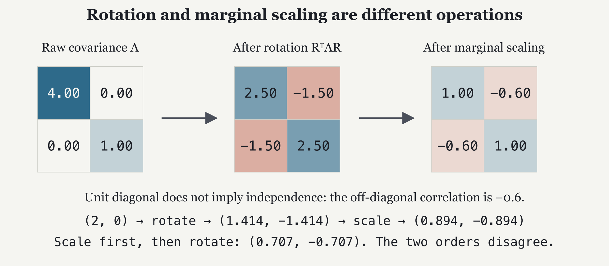
Marginal standardization gives each coordinate unit variance separately. Whitening would also make the covariance between different coordinates zero; we will see that these are different operations. In this illustration only, use two raw directions with variances 4 and 1. Rotate them by 45 degrees using the following $2\times2$ matrix:

$$R=\frac1{\sqrt2}\begin{pmatrix}1&-1\\1&1\end{pmatrix}.$$

Write $\operatorname{Cov}(z)$ for the feature covariance matrix of the standardized article rows in this illustration. Both rotated coordinates have variance 2.5, but they also have covariance -1.5. Divide both by $\sqrt{2.5}$ and their variances become 1 while their covariance becomes -0.6:

$$\operatorname{Cov}(z)=\begin{pmatrix}1&-0.6\\-0.6&1\end{pmatrix}.$$

They now have the same marginal scale. They still move together. Correlation is covariance divided by the two standard deviations; when both variances are one, the correlation equals the covariance. Full whitening would remove these off-diagonal correlations. This pipeline performs marginal standardization, not full whitening.

For the raw row $(2,0)$, rotating and then marginally scaling gives approximately $(0.894,-0.894)$. Scaling the raw coordinates first by $(2,1)$ and then rotating gives $(0.707,-0.707)$. The two operations answer different questions. Their order must be part of the model definition.

This also changes the geometry in which people are compared. Equal lengths in standardized news units need not be equal lengths in the original embedding. A Mahalanobis statistic measures squared distance from a reference mean while accounting for covariance, not just each coordinate’s separate scale. The sum $\sum_jz_j^2$ is not generally that original statistic; see the Eigen Times section on residuals and T squared. Outside this two-dimensional illustration, the symbols retain their fitted-model meanings.

Check 3. Does a covariance matrix with ones on its diagonal necessarily describe uncorrelated coordinates? Use the two-dimensional example to answer.

3.4.1 Unroll the rotation arithmetic

Write the raw coordinate covariance as $\operatorname{diag}(4,1)$, where $\operatorname{diag}$ constructs a diagonal matrix from its listed entries. In the displayed rotation, the first named coordinate is the sum of the two raw coordinates divided by $\sqrt2$; the second is their difference, with the first raw coordinate negative, divided by $\sqrt2$.

Because the raw coordinates have zero covariance, the first named variance is $4(1/\sqrt2)^2+1(1/\sqrt2)^2=2+0.5=2.5$. The second uses the squared negative coefficient and has the same variance. Their covariance uses paired, unsquared coefficients: $4(1/\sqrt2)(-1/\sqrt2)+1(1/\sqrt2)(1/\sqrt2)=-2+0.5=-1.5$. Dividing the two named coordinates by $\sqrt{2.5}$ divides this covariance by $\sqrt{2.5}\sqrt{2.5}=2.5$, leaving $-1.5/2.5=-0.6$.

The row $(2,0)$ first rotates to $(\sqrt2,-\sqrt2)$ and then scales to $(\sqrt{2/2.5},-\sqrt{2/2.5})$. Scaling first instead gives $(1,0)$ and rotating gives $(1/\sqrt2,-1/\sqrt2)$. These routes standardize relative to different coordinate systems, so they use different fitted scale matrices and define different maps. The named-coordinate scale here is a scalar multiple of the identity and actually commutes with the rotation. This example therefore does not test noncommutation of one fixed pair of matrices; each standardizer belongs to the coordinates whose variances it measures.